
Quantum field theory 2, lecture 14
Simplified vertices for homogeneous fields
For homogeneous background fields, and working from now on in Feynman gauge where \(\xi=1\), the gluon vertex terms simplify substantially to \[\begin{split} V_1^{\mu\nu} & = - 2 \mathbf{A}_\rho p^\rho \eta^{\mu\nu}, \\ %+ (1-1/\xi) [\mathbf{A}^\mu p^\nu + \mathbf{A}^\nu p^\mu], \\ V_2^{\mu\nu} & = \mathbf{A}^\rho \mathbf{A}_\rho \eta^{\mu\nu}, \\ %- (1-1/\xi) \mathbf{A}^\mu \mathbf{A}^\nu, \\ V_J^{\mu\nu} & = 2 \mathbf{F}^{\rho\sigma} (J_{\rho\sigma})^{\mu\nu}. \end{split}\] Here \(p^\mu\) is the gluon momentum running through the loop. Similarly, the ghost vertices become \[\begin{split} V_1 & = - 2 \mathbf{A}_\rho p^\rho,\\ V_2 & = \mathbf{A}^\rho \mathbf{A}_\rho. \end{split}\] With this we may proceed with the loop calculation.
Loops with four single legs
We start by considering loop diagrams with four single legs. There is a gluon loop and a ghost loop, where the latter contributes with a negative sign because it is fermionic.
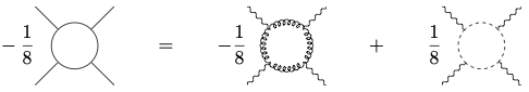
We find in Feynman gauge \[\begin{split} & -\frac{1}{8} \text{tr} \left\{ \mathbf{A}_{\mu_1} \cdots \mathbf{A}_{\mu_4} \right\} \int_p 2 p^{\mu_1} 2 p^{\mu_2} 2 p^{\mu_3} 2 p^{\mu_4} \frac{\delta^\rho_{~\rho}}{(p^2)^4}\\ & +\frac{2}{8} \text{tr} \left\{ \mathbf{A}_{\mu_1} \cdots \mathbf{A}_{\mu_4} \right\} \int_p 2 p^{\mu_1} 2 p^{\mu_2} 2 p^{\mu_3} 2 p^{\mu_4} \frac{1}{(p^2)^4} \end{split}\] The second loop is from ghosts and has an additional minus sign for Grassmann fields and a factor \(2\) for involving complex instead of real fields. The trace over Lorentz indices in the first diagram gives a factor \(d=4\).
Combining the diagrams gives \[- \frac{(4-2)}{8} \text{tr} \left\{ \mathbf{A}_{\mu_1} \cdots \mathbf{A}_{\mu_4} \right\} \int_p \left\{ \frac{2p^{\mu_1}}{p^2} \cdots \frac{2p^{\mu_4}}{p^2} \right\}\] The momentum integral is of a structure that can be simplified based on rotation invariance, \[\begin{split} &\int \frac{d^dp}{(2\pi)^d}~p^{\mu_1}p^{\mu_2}p^{\mu_3}p^{\mu_4} f(p^2)\\ &= \frac{1}{d(d+2)} \left[ \eta^{\mu_1\mu_2}\eta^{\mu_3\mu_4}+\eta^{\mu_1\mu_3}\eta^{\mu_2\mu_4}+\eta^{\mu_1\mu_4}\eta^{\mu_2\mu_3} \right] \int \frac{d^d p}{(2\pi)^d}~p^4 f(p^2). \end{split}\] This leads to a relatively simple result for these two diagrams in \(d=4\) dimensions, \[- \frac{1}{6} \text{tr}\{ \mathbf{A}^\mu \mathbf{A}^\nu \mathbf{A}_\mu \mathbf{A}_\nu + 2 \mathbf{A}^\mu \mathbf{A}_\mu \mathbf{A}^\nu \mathbf{A}_\nu \}\int_p \frac{1}{p^4}.\]
Loops with two single legs and one double leg
Let us now adress the diagrams with two single and one double field vertex. We count also \(V_J\) as a double field vertex.
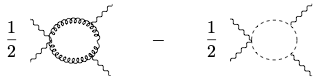
We find here after performing the trace over Lorentz indices in the gluon diagram and subtracting the ghost diagram \[\begin{split} &= \frac{1}{2}\text{tr}\left\{ \mathbf{A}^\rho \mathbf{A}_\rho \mathbf{A}_\mu \mathbf{A}_\nu \right\} (4-2) \int_p \left\{ 2p^\mu 2 p^\nu \frac{1}{(p^2)^3} \right\}. \end{split}\] There is no contribution from the vertex \(V_J^{\mu\nu}\) because it is anti-symmetric in the Lorentz indices. Using \[\begin{split} \int \frac{d^4p}{(2\pi)^4} p^\mu p^\nu f(p^2) = \frac{1}{d} \eta^{\mu\nu} \int \frac{d^4p}{(2\pi)^4}p^2f(p^2) \end{split}\] leads for \(d=4\) to \[\text{tr}\{ \mathbf{A}^\mu \mathbf{A}_\mu \mathbf{A}^\nu \mathbf{A}_\nu \} \int_p \frac{1}{p^4}.\]
Loops with two double legs
Finally we also have diagrams with two double legs.
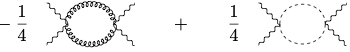
Here we obtain \[\begin{split} & -\frac{1}{4}\text{tr}\left\{ \mathbf{A}^\mu \mathbf{A}_\mu \mathbf{A}^\nu \mathbf{A}_\nu \right\} (4-2) \int_p \frac{1}{p^4} \\ & - \frac{1}{4}\text{tr}\left\{ \mathbf{F}^{\mu\nu} \mathbf{F}^{\rho\sigma} \right\} (J_{\mu\nu})^{\alpha\beta} (J_{\rho\sigma})_{\beta\alpha} \int_p \frac{1}{p^4}. \end{split}\] where the last line is a contribution from the \(V_J^{\mu\nu}\) vertices. We can calculate explicitly \[\begin{split} (J_{\mu\nu})^{\alpha\beta} (J_{\rho\sigma})_{\beta\alpha} = 2 \left[\eta_{\mu\rho} \eta_{\nu\sigma} - \eta_{\mu\sigma} \eta_{\nu\rho}\right]. \end{split}\] This allows to combine the two terms to \[\begin{split} - \frac{1}{2}\text{tr}\{ \mathbf{A}^\mu \mathbf{A}_\mu \mathbf{A}^\nu \mathbf{A}_\nu \} \int_p \frac{1}{p^4} -\text{tr}\{ \mathbf{F}^{\mu\nu} \mathbf{F}_{\mu\nu} \} \int_p \frac{1}{p^4}. \end{split}\]
Combination of all diagrams
We can now combine all gluon and ghost diagrams \[\begin{split} \left[ \frac{1}{6}\text{tr}\left\{\mathbf{A}^\mu \mathbf{A}_\mu \mathbf{A}^\nu \mathbf{A}_\nu \right\} - \frac{1}{6} \text{tr}\left\{ \mathbf{A}^\mu \mathbf{A}^\nu \mathbf{A}_\mu \mathbf{A}_\nu \right\} -\text{tr}\left\{ \mathbf{F}^{\mu\nu} \mathbf{F}_{\mu\nu} \right\}\right]\int_p \frac{1}{p^4}. \end{split}\] Here it is useful to recall that for homogeneous fields one has \[\text{tr}\{ \mathbf{F}^{\mu\nu} \mathbf{F}_{\mu\nu} \} = \text{tr}\{ -2 \mathbf{A}^\mu \mathbf{A}^\nu \mathbf{A}_\mu \mathbf{A}_\nu + 2 \mathbf{A}^\mu \mathbf{A}_\mu \mathbf{A}^\nu \mathbf{A}_\nu \}.\] This allows to combine everything into \[-\frac{11}{12}\text{tr}\{\mathbf{F}^{\mu\nu} \mathbf{F}_{\mu\nu} \} \int_p \frac{1}{p^4}.\] This is almost what we were looking for. We need to remember here, however, that the field strengths are in the adjoint representation. We can remedy this, using an identify for adjoint and fundamental \(\text{SU}(N)\) Lie algebra generators, \[\text{tr} \{ T_u^{(A)} T_v^{(A)} \} = N \delta_{uv} = 2N \text{tr} \{ T_u T_v \}.\]
One-loop quantum effective action
We thus find for the quantum effective action including the one-loop term \[\begin{split} \Gamma[A] = \int_x \left\{ \frac{1}{2\bar g^2} - \frac{11N}{6}\int_p \frac{1}{p^4}\right\} \text{tr} \{ \mathbf{F}^{\mu\nu} \mathbf{F}_{\mu\nu} \}. \end{split}\] Here the field strength is in the fundamental representation as usual, and \(\bar g\) is the microscopic or bare coupling constant.
Finally, we note that the momentum integral is logarithmically divergent both in the UV and in the IR in \(d=4\) dimensions, but can be regularized easily \[\begin{split} \int_p \frac{1}{p^4} = \frac{1}{(2\pi)^4}2\pi^2 \int_0^\infty \frac{dp}{p} \to \frac{1}{(4\pi)^2} 2 \int_\mu^\Lambda \frac{dp}{p} = \frac{2}{(4\pi)^2}\ln \left( \frac{\Lambda}{\mu} \right) \end{split}\] We have introduced a UV cutoff \(\Lambda\) and and IR cutoff \(\mu\).
Running coupling constant
We find the effective coupling constant \(g\) with quantum corrections (one loop) to obey \[\frac{1}{g^2} = \frac{1}{\bar{g}^2}- \frac{11N}{3} \frac{1}{(4\pi)^2}2\ln \left( \frac{\Lambda}{\mu} \right).\] In particular, the effective coupling constant depdends on the infrared regulator scale \(\mu\)!
If we would have done the calculation at non-vanishing external momenta, a corresponding scale would have appeared instead of \(\mu\) naturally. Renormalized coupling constants are scale-dependent as a consequence of quantum fluctuatuions! For Yang-Mills theory, such quantum fluctuations are particularly important because the gluons are massless.
The logarithmic derivative of the coupling constant with respect to the infrared scale is called the beta function, \[\mu \frac{\partial}{\partial \mu} g = \beta(g) = - \frac{g^3}{(4\pi)^2} \left[ \frac{11}{3}N \right].\] This is in fact the renormalization group equation for the coupling constant of \(SU(N)\) gauge theory at one loop, and so far without fermions in the adjoint representation.
More generally, for \(\text{SU}(N)\) gauge theory, with \(n_f\) massless Dirac fermions in the fundamental representation, the beta function is \[\beta(g) = - \frac{g^3}{(4\pi)^2}\left[ \frac{11}{3} N - \frac{2}{3} n_f \right].\] Specifically for QCD, one has \(N=3\), and at high energies where all quarks can be counted massless, \(n_f=6\). The beta function is then \[\beta(g) = - \frac{g^3}{(4\pi)^2}\left[11-4 \right].\]
Asymptotic freedom
A very interesting property of non-Abelian gauge theories is that for small enough \(n_f\), the beta function is negative, \(\beta(g)<0\). This implies that the coupling becomes weaker at higher momentum scale!
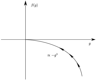
The coupling constant flows into a fixed point at \(g=0\). This property is called asymptotic freedom. At asymptotically large momenta, the theory becomes free.
While QCD as a quantum field theory becomes non-interacting or free at very high energies, the renormalization group beta function also tells that it becomes very strongly interacting at small energies, or in the infrared regime.
Solution to one-loop flow equation*
In terms of the combination \[\alpha_s = \frac{g^2}{4\pi}\] we obtain \[\mu^2\frac{\partial}{\partial\mu^2} \alpha_s(\mu) = \frac{\alpha_s(\mu)^2}{4\pi} \left[ \frac{11}{3}N-\frac{2}{3}n_f \right],\] or \[\mu^2 \frac{\partial}{\partial \mu^2} \left(\frac{4\pi}{\alpha_2}\right) = - \left[ \frac{11}{3}N-\frac{2}{3}n_f \right].\] This can be easily solved, \[\frac{4\pi}{\alpha_s(\mu)} - \frac{4\pi}{\alpha_s(\Lambda)} = \left[ \frac{11}{3}N-\frac{2}{3}n_f \right] \ln\left( \mu^2 / \Lambda^2 \right)\] Imagine we start with some coupling \(\alpha_s(\mu)\) at a scale \(\mu\) and take \(\Lambda\) to be smaller and increase the ratio \(\mu^2/\Lambda^2\). The coupling \(\alpha_s(\Lambda)\) becomes larger and larger until a divergence \(\alpha_s(\Lambda)\to \infty\) some scale, which is by convention called \(\Lambda_\text{QCD}\). We find the solution to the one-loop flow equation \[\alpha_s(\mu) = \frac{4\pi}{\left[ \frac{11}{3}N-\frac{2}{3}n_f \right] \ln\left( \mu^2 / \Lambda_\text{QCD}^2 \right)}.\] One should keep in mind that perturbation theory breaks down when \(\alpha_s\) becomes too large. It is only applicable at large energies \(\mu\gg \Lambda_\text{QCD}\).