Quantum field theory 2, lecture 13

Quadratic part in fluctuation gauge fields

To calculate \(S^{(2)}[A]\), we specifically need the term quadratic in \(\mathbf{a}_\mu'(x)\). Collecting terms from the Yang-Mills action we find \[\begin{split} S_2 = & \int_x \frac{1}{2g^2}\text{tr}\left\{(D^\mu[A] \mathbf{a}^{\prime\nu}(x)-D^\nu[A] \mathbf{a}^{\prime\mu}(x))(D_\mu[A] \mathbf{a}_\nu'(x)-D_\nu[A] \mathbf{a}_\mu'(x)) \right.\\ & \left. \quad\quad\quad\quad\quad\quad -2i \bar{\mathbf{F}}^{\mu\nu}_\text{fnd}(x) [\mathbf{a}^\prime_\mu(x) , \mathbf{a}^\prime_\nu(x) ] \right\} \\ = & \int_x \frac{1}{g^2}\text{tr}\left\{ \mathbf{a}_\mu'(x) \left[ -\eta^{\mu\nu} D^\rho[A] D_\rho[A] + D^\nu[A] D^\mu[A] +i \bar{\mathbf{F}}^{\mu\nu}_\text{adj}(x) \right] \mathbf{a}_\nu'(x) \right\}. \end{split}\] In the second equation we performed partial integrations and used an identify following from the cyclic property of the trace, \[\begin{split} \frac{-i}{g^2}\text{tr}\{ \bar{\mathbf{F}}^{\mu\nu}_\text{fnd}(x) [\mathbf{a}^\prime_\mu(x) , \mathbf{a}^\prime_\nu(x) ] \} = & \frac{i}{g^2} \, \text{tr} \left\{ \mathbf{a}^\prime_\mu(x) \left[\bar{\mathbf{F}}^{\mu\nu}_\text{fnd}(x) , \mathbf{a}^\prime_\nu(x) \right] \right\} \\ = & \frac{i}{g^2} \text{tr} \left\{ \mathbf{a}^\prime_\mu(x) \bar{\mathbf{F}}^{\mu\nu}_\text{adj}(x) \mathbf{a}^\prime_\nu(x)\right\}. \end{split}\] One may also use \[D^\nu[A] D^\mu[A] = D^\mu[A] D^\nu[A] + \left[ D^\nu[A], D^\mu[A] \right] = D^\mu[A] D^\nu[A] +i \bar{\mathbf{F}}^{\mu\nu}\] where all covariant derivatives and the field strength tensor are in the adjoint representation of the Lie algebra.

Combining terms, and adding now also the gauge fixing term leads to \[\begin{split} S_2 = & \int_x \frac{1}{g^2}\text{tr}\left\{ \mathbf{a}_\mu'(x) \left[ -\eta^{\mu\nu} D^\rho[A] D_\rho[A] + (1-1/\xi) D^\mu[A] D^\nu[A] +2 i \bar{\mathbf{F}}^{\mu\nu} \right] \mathbf{a}_\nu'(x) \right\} \\ = & \int_x \frac{1}{2}\left\{ a_{z \mu}^{\prime}(x) [-\eta^{\mu\nu} D^\rho[A] D_\rho[A]+ (1-1/\xi)D^\mu[A] D^\nu[A] +2 i \bar{\mathbf{F}}^{\mu\nu}(x) ]^z_{~w} a_\nu^{\prime w}(x) \right\} \end{split}\] In the second equation we used \(\text{tr}(T_zT_w) = \delta_{zw}/2\) as well as \(\mathbf{a}_\mu^\prime(x) = g a_\mu^{\prime w}(x) T_w\) This is finally the form we use in the following.

Expanding the inverse gluon propagator

It is useful to decompose the inverse gluon propagator in the presence of background field into different terms \[\begin{split} & [-\eta^{\mu\nu} D^\rho[A] D_\rho[A]+ (1-1/\xi)D^\mu[A] D^\nu[A] +2 i \bar{\mathbf{F}}^{\mu\nu}(x) ]^z_{~w} \\ & = [ P^{\mu\nu} + V_1^{\mu\nu} + V_2^{\mu\nu} + V_J^{\mu\nu}]^z_{~w}. \end{split}\] Here the leading term is the free inverse propagator \[P^{\mu\nu} = -\eta^{\mu\nu}\partial^\rho\partial_\rho+(1-1/\xi)\partial^\mu \partial^\nu,\] which is easily inverted in momentum space, leading to the free gluon propagator \[\frac{\eta_{\mu\nu}-(1-\xi)p_\mu p_\nu/p^2}{p^2}.\] We also have a term linear in the background gauge field \[\begin{split} V_1^{\mu\nu} = & i [\partial^\rho \mathbf{A}_\rho(x)] \eta^{\mu\nu}+ 2 i \mathbf{A}^\rho(x)\partial_\rho \eta^{\mu\nu}\\ & - i (1-1/\xi) [\partial^\mu \mathbf{A}^\nu(x)] - i (1-1/\xi) [\mathbf{A}^\mu(x) \partial^\nu + \mathbf{A}^\nu(x) \partial^\mu] \end{split}\] The gauge fields \(\mathbf{A}_\rho(x)\) are here in the adjoint representation. This corresponds to a vertex couling the background field to a gluon line. A similar term is quadratic in the background field, \[V_2^{\mu\nu} = \mathbf{A}^\rho(x) \mathbf{A}_\rho(x) \eta^{\mu\nu} - (1-1/\xi) \mathbf{A}^\mu(x) \mathbf{A}^\nu(x).\] Finally, there is a term linear in the background field strength, which is best written as \[V_J^{\mu\nu} = 2 \mathbf{F}^{\rho\sigma}(x) (J_{\rho\sigma})^{\mu\nu},\] with \[(J_{\rho\sigma})^{\mu\nu} = i(\delta_{\rho}^\mu \delta_\sigma^\nu - \delta_\rho^\nu\delta_\sigma^\mu),\] being the generator of Lorentz transformations in the vector representation. This corresponds to a vertex directly coupling to the background field strength.

Quadratic part in ghost fields and inverse propagator

We also need the quadratic part of the ghost action, \[S_2 = \int_x \bar{c}_z(x)[-D^\rho[A] D_\rho[A]]^z_{~w} c^w(x).\] The inverse propagator can be expanded similar as for the gluons, \[D_\rho[A]]^z_{~w} = [P + V_1 + V_2]^z_{~w},\] with the inverse free ghost propagator \[P = -\partial^\rho \partial_\rho,\] which can be inverted in momentum space to \(1/p^2\). The vertices are \[V_1 = i [\partial^\rho \mathbf{A}_\rho(x)] + 2 i \mathbf{A}^\rho(x)\partial_\rho,\] and \[V_2 = \mathbf{A}^\rho(x) \mathbf{A}_\rho(x),\] with all background gauge fields in the adjoint representation.

Field expansion of one-loop action

We now discuss a general method to expand a one-loop expressions in terms of fields. Generically, the inverse propagator is of the form \[S^{(2)} = \mathscr{P} + \mathscr{F}_1 + \mathscr{F}_2 + \ldots.\] Here \(\mathscr{P}\) is independent of the fields, \(\mathscr{F}_1\) is linear in field, \(\mathscr{F}_2\) is quadratic and so on. Usually one can invert \(\mathscr{P}\) by going to momentum space, and we denote here \[\mathscr{G} = \mathscr{P}^{-1}.\] Consider now a one-loop expression \[\begin{split} \frac{1}{2}\text{STr}\{\ln S^{(2)} \} = & \frac{1}{2}\text{STr}\left\{\ln \left(\mathscr{P}+\mathscr{F}_1+\mathscr{F}_2+\ldots \right) \right\} \\ = & \frac{1}{2} \text{STr} \left\{ \ln(\mathscr{P}) \right\} + \frac{1}{2} \text{STr} \left\{ \ln\left( 1 + \mathscr{G} \mathscr{F}_1 + \mathscr{G} \mathscr{F}_2 + \ldots \right) \right\}. \end{split}\] Here one can expand the logarithm, which yields \[\begin{split} \frac{1}{2}\text{STr}\{\ln S^{(2)}\} &= \frac{1}{2}\text{STr}\{\ln(\mathscr{P}) \} + \frac{1}{2} \text{STr}\left\{\mathscr{G}\mathscr{F}_1+\mathscr{G}\mathscr{F}_2 + \ldots \right\}\\ &\quad - \frac{1}{4}\text{STr}\left\{\mathscr{G}\mathscr{F}_1 \mathscr{G}\mathscr{F}_1 +2\mathscr{G}\mathscr{F}_1 \mathscr{G} \mathscr{F}_2 + \mathscr{G} \mathscr{F}_2 \mathscr{G}\mathscr{F}_2 + \ldots \right\}\\ &\quad + \frac{1}{8}\text{STr}\{\mathscr{G}\mathscr{F}_1 \mathscr{G}\mathscr{F}_1\mathscr{G}\mathscr{F}_1 +3\mathscr{G}\mathscr{F}_1 \mathscr{G} \mathscr{F}_1 \mathscr{G}\mathscr{F}_2 + \ldots \}\\ &\quad - \frac{1}{8}\text{STr}\{\mathscr{G}\mathscr{F}_1 \mathscr{G}\mathscr{F}_1\mathscr{G}\mathscr{F}_1\mathscr{G}\mathscr{F}_1+\ldots \} \end{split}\] The terms on the left hand side have a diagrammatic interpretation. The first term is independent of the background field and contributes only to the constant part of the effective action. The subsequent terms are loop expressions with external background field insertions.

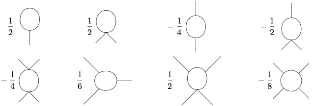
Specifically, we kept here all terms with up to four external fields while higher orders have been suppressed.

Projection to field strength squared term

The effective action \(\Gamma[A]\) contains not only the term proportional to \(\text{tr}\{\mathbf{F}^{\mu\nu} \mathbf{F}_{\mu\nu}\}\), but also many other structures allowed by the symmetries. In order to project to the coefficient of this term, we could determine the coefficient of the term quadratic, of the term cubic, or of the term quartic in the background gauge field in \(\text{tr}\{\mathbf{F}^{\mu\nu}\mathbf{F}_{\mu\nu}\}\). We follow here the last strategy, but gauge invariance implies that all these coefficients must actually be equal.

Note that \[\begin{split} \int_x \frac{1}{2g^2}\text{tr}\left\{\mathbf{F}^{\mu\nu}(x) \mathbf{F}_{\mu\nu}(x) \right\} = \ldots + \int_x \frac{1}{2g^2} \text{tr}\{ - [\mathbf{A}^\mu(x), \mathbf{A}^\nu(x)] [\mathbf{A}_{\mu}(x), \mathbf{A}_\nu(x)] \}. \end{split}\] Because the right hand side contains no derivatives, we can evaluate it in momentum space at vanishing momentum, or, in other words, for homogeneous backgound fields \(\mathbf{A}_\mu(x) = \mathbf{A}_\mu\).