Quantum field theory 2, lecture 15

Wegner-Wilson loops and confinement

Wilson links

Let us consider pure Yang-Mills theory (without quarks) with the Euclidean action \[S_\text{Yang-Mills}[A] = \int_x \left\{\frac{1}{2g^2} \text{tr}\left\{\mathbf{F}^{\mu\nu}(x) \mathbf{F}_{\mu\nu}(x)\right\} \right\}.\] Let us take two spacetime points \(x^\mu\) and \(x^\mu + \varepsilon^\mu\) where \(\varepsilon^\mu\) is infinitesimal. We define the Wilson link as \[\begin{split} \mathbf{W}(x+\varepsilon,x) &= \exp\left(i \varepsilon^\mu \mathbf{A}_\mu (x) \right) \\ &= \mathbb{1} + i\varepsilon^\mu \mathbf{A}_\mu(x) + \mathcal{O}(\varepsilon^2). \end{split}\] Because \(\mathbf{A}_\mu(x)\) is an \(N\times N\)-matrix, this is also the case for \(\mathbf{W}(x+\varepsilon,x)\). We now determine how the Wilson link transforms under gauge transformations. Recall the finite gauge transformations for the fermion and gauge fields, \[\begin{split} \psi(x) &\to U(x) \psi(x),\\ \mathbf{A}_\mu(x) &\to U(x) \mathbf{A}_\mu(x) U^\dagger(x) - i [\partial_\mu U(x)] U^\dagger(x). \end{split}\] The Wilson link (to order \(\varepsilon\)) transforms as \[\begin{split} \mathbf{W}(x+\varepsilon,x) &\to \mathbb{1} + i\varepsilon^\mu U(x) \mathbf{A}_\mu(x) U^\dagger (x) + \varepsilon^\mu [\partial_\mu U(x)] U^\dagger(x). \end{split}\] Here one can use that to order \(\varepsilon\), \[U(x+\varepsilon) = U(x) + \varepsilon^\mu \partial_\mu U(x).\] Accordingly we obtain a simple transformation law, \[\mathbf{W}(x+\varepsilon,x)\to U(x+\varepsilon) \mathbf{W}(x+\varepsilon,x) U^\dagger(x).\] This indicates the geometric significance of the Wilson link as connecting the gauge groups at different points in space-time.

Wilson line

We can now consider a Wilson line as a chain of infinitesimal Wilson links. It goes along some path \(\xi\), connecting two spacetime points \(x\) and \(y=x+\varepsilon_1 + \cdots + \varepsilon_n\), \[\begin{split} \mathbf{W}_\xi(y,x) = \mathbf{W}(y,y-\varepsilon_n) \cdots \mathbf{W}(x+\varepsilon_1 + \varepsilon_2,x+\varepsilon_1) \mathbf{W}(x+\varepsilon_1,x). \end{split}\] The transformation behaviour under gauge transformations is rather simple, \[\mathbf{W}_\xi(y,x) \to U(y) \mathbf{W}_\xi (y,x) U^\dagger(x).\] For a Wilson link, one can write \[\begin{split} \mathbf{W}^\dagger(x+\varepsilon,x) = \mathbf{W}(x,x+\varepsilon). \end{split}\] For a finite Wilson line, this extends to \[\mathbf{W}_\xi^\dagger(y,x) = \mathbf{W}_{\bar{\xi}}(x,y),\] where \(\bar{\xi}\) denotes the reverse of the path \(\xi\).

Wegner-Wilson loop

Consider now a closed path or oriented curve \(\xi = \mathcal{C}\). The Wegner-Wilson loop is the trace of the Wilson line along the closed curve, \[W_\mathcal{C} = \text{tr}\{ \mathbf{W}_\mathcal{C}(x,x) \}.\] The trace goes over the \(\text{SU}(N)\) matrix indices and the Wilson loop is accordingly not a matrix but a scalar.

Note that the Wegner-Wilson loop depends on the entire path of the loop and is in this sense not a local field of a standard type.

From the transformation law of the Wilson line, it follows that the Wegner-Wilson loop is gauge invariant, \[W_\mathcal{C} \to W_\mathcal{C}.\] Furthermore, the complex conjugate is \[\begin{split} W_\mathcal{C}^* = W_{\bar{\mathcal{C}}}, \end{split}\] with reversed path \(\bar{\mathcal{C}}\).

Interaction potential from Wegner-Wilson loop

One may obtain the interaction potential between two very heavy or static particles from the Wegner-Wilson loop. To this end, consider a rectangular closed path with lengths \(T\) in euclidean time and \(R\) in space direction, such that \(T \gg R\). When \(\langle W_{\mathcal{C}}\rangle\) is computed, we are actually solving the functional integral in the presence of static, opposite charges with separation \(R\). The Euclidean path integral will then be proportional to \(\exp(-E(R)T)\), where \(E(R)\) is the interaction energy of the two heavy particles.

QED or weak coupling expansion

Let us consider the expectation value of the Wegner-Wilson loop in the Abelian theory (QED). A weak-coupling expansion of Yang-Mills theory leads to a very similar theory.

One can write \[\begin{split} \langle W_{\mathcal{C}} \rangle &= \int D A \exp\left( i g \int_{\mathcal{C}} dx^\mu A_\mu(x) \right) \exp\left(-S[A]\right). \end{split}\] The line integral in the exponential has the form of a current term in the partition function, \[\exp\left( \int_x \{ j^\mu(x) A_\mu(x)\}\right),\] if we write the current in the form of a line integral, \[j^\mu(x) = ig \int_{\mathcal{C}} d\tilde{x}^\mu \delta^{(4)}(x-\tilde{x}).\] For the free Abelian gauge field, the partition function is quadratic and one finds \[\begin{split} \left\langle \exp\left(\int_x j^\mu(x)A_\mu(x)\right) \right\rangle = \exp\left( \frac{1}{2}\int_{x,y}\left\{ j^\mu(x) \Delta_{\mu\nu}(x-y) j^\nu(y) \right\} \right), \end{split}\] with Euclidean photon propagator \(\Delta_{\mu\nu}(x-y)\). The Wegner-Wilson loop eveluates to \[\langle W_{\mathcal{C}} \rangle = \exp\left( - \frac{g^2}{2}\int_{\mathcal{C}} dx^\mu \int_{\mathcal{C}} dy^\nu \Delta_{\mu\nu}(x-y) \right).\]

Coulomb potential

Consider now the rectangular configuration with \(T \gg R\). For the photon propagator we can take the Feynman gauge expression (in \(d=4\) Euclidean dimensions) \[\Delta_{\mu\nu}(x-y) = \frac{\delta_{\mu\nu}}{4\pi^2(x-y)^2}.\] Doing the integrals (exercise) one finds with \(\alpha=g^2/(4\pi)\), \[\begin{split} \langle W_{\mathcal{C}}\rangle =\text{const} \times \exp\left( - \frac{\alpha}{R}T \right). \end{split}\] The constant part is in fact divergent and corresponds to the infinite self energy of a classical charged particle. From the \(R\)-dependece, one can read off the static potential \(V(R)=-\alpha/R\). This is Coulombs potential.

In a weak coupling expansion of a non-abelian gauge theory like QCD, one also finds the Coulomb potential. However this cannot be the full story. We now describe a strong coupling expansion for the Wegner-Wilson loop.

Wegner-Wilson plaquette

Imagine that we formulate the gauge theory on a discrete spacetime lattice with lattice spacing \(a\). We now consider a Wilson loop of the form

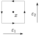
going around a point \(x\). The gauge fields and link variables are in the lattice formulation living between the lattice sites. With two space-time vectors \(\varepsilon_1\) and \(\varepsilon_2\) of length \(a\), we use the link variables at \(x\pm \varepsilon_1/2\) and \(x\pm\varepsilon_2/2\) to formulate a discrete version of the Wegner-Wilson loop. We define this loop to be the plaquette. Multiplying the Wilson links around the loop and taking the trace gives the Wegner-Wilson loop \[W_{\text{plaq}} = \text{Tr}\left\{ e^{-ia \mathbf{A}_2(x- \frac{\varepsilon_1}{2})} e^{-ia \mathbf{A}_1( x+ \frac{\varepsilon_2}{2})} e^{ ia \mathbf{A}_2( x+ \frac{\varepsilon_1}{2})} e^{ ia \mathbf{A}_1( x- \frac{\varepsilon_2}{2})} \right\}.\] Assume now that the gauge fields are smooth and expand to quadratic order in the lattice spacing \(a\), \[\begin{split} W_{\text{plaq}} = \text{Tr} & \bigg\{ e^{-ia \mathbf{A}_2(x) + ia^2 \partial_1 \mathbf{A}_2(x)/2 } e^{-ia \mathbf{A}_1(x) - ia^2 \partial_2 \mathbf{A}_1(x)/2 } \\ & \times e^{ ia \mathbf{A}_2(x) + ia^2 \partial_1 \mathbf{A}_2(x)/2 }~ e^{ ia \mathbf{A}_1(x) - ia^2 \partial_2 \mathbf{A}_1(x)/2 } \bigg\}. \end{split}\] With help of the Bakeer-Campbell-Hausdorff relation \[e^A e^B = e^{A+B+[A,B]/2+\ldots},\] one can combine the exponentials in the first line and in the second line and then both lines together. The result is \[\begin{split} W_{\text{plaq}} &= \text{Tr}\left\{ e^{ia^2 (\partial_1 \mathbf{A}_2-\partial_2 \mathbf{A}_1-i[\mathbf{A}_1,\mathbf{A}_2])} \right\} = \text{Tr} \left\{ e^{ia^2 \mathbf{F}_{12}} \right\}. \end{split}\] We see the non-Abelian field strength naturally appearing! The Wilson loop of the same plaquette in the opposite sense gives \[W_{\overline{\text{plaq}}} = \text{Tr}\left\{ e^{-ia^2 (\partial_1 \mathbf{A}_2-\partial_2 \mathbf{A}_1-i[\mathbf{A}_1,\mathbf{A}_2])} \right\} = \text{Tr} \left\{ e^{-ia^2 \mathbf{F}_{12}} \right\}.\]