Quantum field theory 2, lecture 11

Functional integral for gauge theories

The following discussion will be given in the Euclidean domain formulation of the theory, but works similarly in Minkwoski space. In other words, we work with the Euclidean action \(S_\text{E}\), but for simplicity we drop the index E.

Let us try to proceed with the standard definition \[\begin{split} Z[j] = \int DA ~\exp\left(-S[A]+\int_x\left\{ A_\mu^z(x)j_z^\mu(x)\right\}\right). \end{split}\] The functional integral contains an integral over the gauge modes that are the extension of the longitudinal gauge bosons to the whole space of non-Abelian gauge fields \(A^z_\mu(x)\).

The action does not depend on the gauge modes. As a consequence, the functional integral diverges. Furthermore, perturbation theory cannot be used. In other words, \(S^{(2)}\) is not invertible, and we cannot proceed by a saddle point expansion.

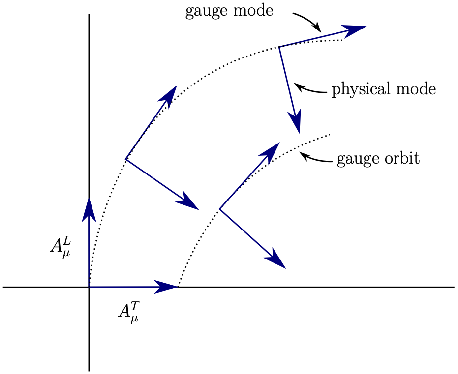
Gauge fixing in Abelian gauge theory

Gauge fixing term

For an Abelian theory, we can define a global physical field \(A_\mu^T(x)\) and a global gauge degree of freedom \(A_\mu^L(x)\). Since the action does not depend on \(A_\mu^L(x)=\partial_\mu\beta(x)\), we may simply “take out” this part from the functional integral by invoking a functional Dirac distribution, \[Z[j] = \int DA~\delta[A_\mu^L] \exp\left(-S[A]+\int_x j^\mu(x) A_\mu(x)\right).\]

We can replace the functional Dirac distribution by a Gaussian, \[\delta[A_\mu^L] \to \lim_{\xi\to 0} \exp\left( - \frac{1}{2\xi}\int_x[\partial^\mu A_\mu(x)]^2 \right).\] Note that when \(A^T_\mu(x)\) obeys the Landau gauge condition, the functional above vanishes except when \(\partial^\mu A_\mu(x) = \partial^\mu\partial_\mu\beta(x)=0\). This is sufficient gauge fixing, at least for perturbation theory.

One may consider the “gauge fixing term” as an addition to the gauge invariant action \(S\), \[Z[j] = \int DA~\exp\left(-S[A]-S_\text{gf}[A]+\int_x\{ j_\text{c}^\mu(x) A_\mu^T(x) \}\right)\] where \[S_\text{gf}[A] = \frac{1}{2\xi}\int_x\left\{\left[\partial^\mu A_\mu(x)\right]^2\right\}.\] We take \(\xi\to0\) at the end. This is called “Landau gauge fixing”.

Propagator with gauge fixing

The gauge fixing term provides an inverse propagator for the longitudinal photon. From \[S_\text{gf}[A] = \frac{1}{2\xi} \int_p A_\nu(-p) p^\nu p^\mu A_\mu(p),\] we infer \[(S_\text{gf}^{(2)})^{\mu\nu}(p,q) = \frac{1}{\xi} q^\mu q^\nu = \frac{1}{\xi} p^2\left[ \delta^{\mu\nu} - \mathscr{P}^{\mu\nu} \right](2\pi)^d \delta^{(d)}(p-q).\] The microscopic or classical inverse propagator with gauge fixing, proportional to \[\eta^{\mu\nu} p^2 + \left[\frac{1}{\xi}-1\right] p^\mu p^\nu,\] is now invertible, with the classical propagator being proportional to \[\frac{1}{p^2} \left[ \eta_{\mu\nu} + (\xi-1) \frac{p_\mu p_\nu}{p^2} \right].\] Now perturbation theory can be developed.

Gauge fixing in non-Abelian gauge theories

Background fluctuation splitting

Let us decompose the non-Abellian gauge field we use as integration variable in the functional integral as \[a^z_\mu(x) = A^z_\mu(x) + a^{\prime z}_\mu(x).\] The field \(A^z_\mu(x)\) is a background field, while \(a^{\prime z}_\mu(x)\) is a fluctuating field. We will eventually do a change of variables and integrate over the field \(a^{\prime z}_\mu(x)\).

Under an inifinitesimal gauge transformation the full field transforms as \[\begin{split} a^z_\mu(x) & \to a_\mu^z(x) + \frac{1}{g}\partial_\mu \alpha^z(x) - \alpha^y(x) f_{yw}^{~~z} a^w_\mu(x) \\ & = a_\mu^z(x) + \frac{1}{g} (D_\mu[a])^z_{~y} \alpha^y(x). \end{split}\] One could distribute this transformation in different ways to the background field \(A_\mu^z(x)\) and fluctuating field \(a^{\prime z}_\mu(x)\). We discuss now two possibilities.

Fluctuation field gauge transform

We first consider a “fluctuation field gauge transform”, where the background part \(A^z_\mu(x)\) is unchanged, and \(a^{\prime z}_\mu(x)\) gets transformed, \[\begin{split} A^z_\mu(x) & \to A^z_\mu(x),\\ a^{\prime z}_\mu(x) & \to a^{\prime z}_\mu(x) + \frac{1}{g}\partial_\mu \alpha^z(x) - \alpha^y(x) f_{yw}^{~~z} \left[A^w_\mu(x) + a^{\prime w}_\mu(x) \right]\\ & = a^{\prime z}_\mu(x) + \frac{1}{g} (D_\mu[A+a^\prime])^z_{~y} \alpha^y(x). \end{split}\] Here the fluctuation field is transforming almost like the full gauge field, just with an additional background being present.

Background field gauge transform

It is also sometimes useful to consider a “background field gauge transform”, where the background field is transformed like a gauge field, \[\begin{split} A^z_\mu(x) & \to A^z_\mu(x) + \frac{1}{g} (D_\mu[A])^z_{~y} \alpha^y(x),\\ a^{\prime z}_\mu(x) & \to a^{\prime z}_\mu(x) + i \alpha^y(x) (T_y^{(A)})z_{~w} a^{\prime w}_\mu(x),\\ & = a^{\prime z}_\mu(x) - \alpha^y f_{yw}^{~~z} a^{\prime w}_\mu(x). \end{split}\] Here the fluctuation field \(a^{\prime z}_\mu(x)\) transforms as a matter field in the adjoint representation of the gauge group! The background field transforms as a proper gauge field, instead.

Rewriting unity

In the following it is useful to have a factor unity written in a particularly convenient way. We start from the familiar identity \[\int dz \, \delta(f(z)) \frac{df(z)}{dz} =1,\] where we assume that \(f(z)\) has a single zero crossing in the relevant range of \(z\) and that \(df(z)/dz\) is positive there. One can generalize this to several variables, \[\left[\prod_{j=1}^N \int dz_j \right] \delta^{(N)}(\mathbf{f}(\mathbf{z})) \det\left( \frac{\partial f_k(\mathbf{z})}{\partial z_j} \right) = 1.\] The determinant of the Jacobi matrix arises from a change of variables in the vicinity of the zero crossing of the vector valued function, \(\mathbf{f}(\mathbf{z})=0\).

In the limit \(N\to \infty\) this idendity generalizes to a functional idendity, \[\begin{split} \int D\alpha~\delta[G[\alpha]]~\text{Det}\left[\tfrac{\delta}{\delta \alpha} G[\alpha]\right] = 1. \end{split}\] For our purpose we use the functional integral over the gauge orbit (the gauge group manifold) at every space-time point, \[\int D\alpha = \prod_x\prod_z\int d\alpha^z(x).\] In the theory of Lie groups, a convenient integral measure is known as the Haar measure.

The functional \(G[\alpha]\) encodes a gauge condition, in the sense that it should vanish when the condition is fulfilled. We write it as \[G^z(x)[A, a^\prime[\alpha]] = 0,\] where \(\alpha^z(x)\) is the parameter field of a fluctuation gauge transform and \(a^\prime[\alpha]\) is the gauge-transformed fluctuation field. It is enough to know \(a^\prime[\alpha]\) for infinitesimal \(\alpha^z(x)\) where it is for the fluctuation field gauge transform \[a^{\prime z}_\mu(x)[\alpha] = a^{\prime z}_\mu(x) + \frac{1}{g}(D_\mu[A+a^\prime])^z_{~y} \alpha^y(x).\] The Jacobi matrix is now a functional derivative, \[N^z_{~w}(x,y)[A,a^\prime[\alpha]] = \frac{\delta}{\delta \alpha^w(y)} G^z(x)[A, a^\prime[\alpha]].\]

Functional interal and inserting unity

Consider now the partition function for Yang-Mills theory, \[\begin{split} Z[j] = e^{W[j]} = & \int D a \exp\left( -S[a] + \int_x \{ j_z^\mu(x) a^z_\mu(x) \} \right) \\ = & \int D a^\prime \exp\left( -S[A+a^\prime] + \int_x \{ j_z^\mu(x) (A_\mu^z(x) + a^{\prime z}_\mu(x)) \} \right) \\ \end{split}\] In the last equation we use the splitting \(a^z_\mu(x) = A_\mu^z(x) + a^{\prime z}_\mu(x)\).

We now insert a factor of unity under the functional integral, \[\begin{split} e^{W[j]} = & \int D a^\prime \int D\alpha \, \delta\left[G[A, a^\prime[\alpha]]\right] \, \text{Det}\left[ \tfrac{\delta}{\delta\alpha} G[A, a^\prime[\alpha]] \right]\\ & \times \exp\left( -S[A+a^\prime] + \int_x \{ j_z^\mu(x) (A_\mu^z(x) + a^{\prime z}_\mu(x)) \} \right). \end{split}\] The gauge condition \(G[A, a^\prime[\alpha]]\) depends on the background field \(A^z_\mu(x)\) and the gauge transformed fluctuation field \(a^{\prime z}_\mu(x)[\alpha]\), with gauge transformation parameter field \(\alpha^z(x)\).

Changing the order of integration and transforming the gauge

In a next step we change the order of the two functional integrals, \[\int D a^\prime \int D\alpha = \int D\alpha \int D a^\prime.\] Moreover, we can use then that the action is actually gauge invariant, such that \[S[A+a^\prime] = S[A+a^\prime[\alpha]].\] The same should hold for the functional integral measure, \[\int D a^\prime = \int D a^\prime[\alpha].\] We assume in addition that we can replace the source term \[\int_x \{ j_z^\mu(x) (A_\mu^z(x) + a^{\prime z}_\mu(x)) \} \to \int_x \{ j_z^\mu(x) (A_\mu^z(x) + a^{\prime z}_\mu(x)[\alpha]) \}\] After all, it is a bit arbitrary whether to introduce a source before or after doing a gauge transformation. This leads us to \[\begin{split} e^{W[j]} = & \int D\alpha \int D a^\prime[\alpha] \, \delta\left[G[A, a^\prime[\alpha]]\right] \, \text{Det}\left[ \tfrac{\delta}{\delta\alpha} G[A, a^\prime[\alpha]] \right]\\ & \times \exp\left( -S[A+a^\prime[\alpha]] + \int_x \{ j_z^\mu(x) (A_\mu^z(x) + a^{\prime z}_\mu(x)[\alpha]) \} \right). \end{split}\]

Relabeling integration variables and dropping gauge orbit integral

Now one observes that \(a^\prime[\alpha]\) appears everywhere, and it is actually an intgration variable. So one may simply relabel it back to \(a^\prime\). This has the interesting consequence that all dependence on \(\alpha^z(x)\) drops out, and the functional integral \(\int D \alpha\) is just a large factor, which can be dropped. One arrives at the expression \[\begin{split} e^{W[j]} = & \int D a^\prime \, \delta\left[G[A, a^\prime]\right] \, \text{Det}\left[ \tfrac{\delta}{\delta\alpha} G[A, a^\prime] \right]\\ & \times \exp\left( -S[A+a^\prime] + \int_x \{ j_z^\mu(x) (A_\mu^z(x) + a^{\prime z}_\mu(x)) \} \right). \end{split}\]

Gauge fixing in generalized Landau gauge

A convenient gauge fixing for \(a^{\prime z}_\mu(x)\) for a given macroscopic field \(A_\mu^z(x)\) is the generalized Landau gauge condition \[\begin{split} G^z(x)[A, a^\prime] = & (D^\mu[A])^z_{~w} a_\mu^{\prime w}(x) \\ = & \partial^\mu a_\mu^{\prime z}(x) + g A^{y\mu} f_{yw}^{~~z} \, a_\mu^{\prime w}(x) = 0. \end{split}\] Here \((D^\mu[A])^z_{~w}\) is the covariant derivative in the adjoint representation.

With this choice we can write the functional Dirac distribution as an exponential, \[\delta[G[A, a^\prime]] = \lim_{\xi\to\infty} \exp\left( - \frac{1}{2\xi} \int_x \left\{ \delta_{uv} (D^\mu[A])^u_{~w} a_\mu^{\prime w}(x)(D^\nu[A])^v_{~z} a^{\prime z}_\nu(x) \right\}\right).\] This adds a gauge fixing term to the action that depends on the background field as well as on the fluctuation field, \[S_\text{gauge fixing}[A,a^\prime] = \int_x \left\{ \frac{\delta_{uv}}{2\xi} (D^\mu[A])^u_{~w} a_\mu^{\prime w}(x)(D^\nu[A])^v_{~z} a^{\prime z}_\nu(x) \right\}.\]