Quantum field theory 2, lecture 10

Commutator of covariant derivatives and field strength

Consider the covariant derivative in some representation of the Lie algebra \[D_\mu = \partial_\mu - i g A_\mu^z(x) T_z = \partial_\mu -i \mathbf{A}_\mu(x).\] In the last equation we introduced a Lie-algebra-valued gauge field \(\mathbf{A}_\mu(x) = g A_\mu^z(x) T_z\). The rescaling by the coupling constant is also convenient. Let us calculate the commutator of the two covariant derivatives, \[\begin{split} [D_\mu,D_\nu] &= \left[\partial_\mu-i\mathbf{A}_\mu(x),\partial_\nu-i\mathbf{A}_\nu(x) \right]\\ &= -i\left(\partial_\mu \mathbf{A}_\nu(x)-\partial_\nu \mathbf{A}_\mu(x) -i\left[\mathbf{A}_\mu(x),\mathbf{A}_\nu(x)\right]\right) \end{split}\] The resulting expression can be seen as a non-Abelian, and Lie-algebra-valued generalization of the field strength tensor, \[\mathbf{F}_{\mu\nu}(x) = \partial_\mu \mathbf{A}_\nu(x)-\partial_\nu \mathbf{A}_\mu(x) -i\left[\mathbf{A}_\mu(x),\mathbf{A}_\nu(x)\right] = g F^z_{\mu\nu}(x) T_z.\] The field strength tensor in components is \[\begin{split} F^z_{\mu\nu}(x) = & \partial_\mu A^z_{\nu}(x) - \partial_\nu A^z_{\mu}(x) + g f_{yw}^{~~z} A^y_\mu(x) A^w_\nu(x). \end{split}\] Note in particular that the field strength contains terms linear and quadratic in the gauge field.

From the definition as a commutator of covariant derivatives one finds that gauge transformations transform the fields strength in a covariant way, \[\mathbf{F}_{\mu\nu}(x) \to U(x) \mathbf{F}_{\mu\nu}(x) U^{-1}(x).\] A combination like \[\frac{1}{2g^2} \text{tr} \left\{ \mathbf{F}^{\mu\nu}(x)\mathbf{F}_{\mu\nu}(x) \right\} = \frac{1}{4} F_z^{\mu\nu}(x) F^z_{\mu\nu}(x)\] is accordingly invariant and can appear in the Lagrangian. We used here \(\text{tr}\{ T_z T_w \}=\delta_{zw}/2\).

Gauge invariant action

We now construct gauge invarant actions and start with a kinetic term for the fermions, \[\begin{split} S_\text{Dirac} = & \int_x \left\{ - \bar \psi(x) \gamma^\mu D_\mu \psi(x) \right\} \\ = & \int_x \left\{ - \bar \psi(x) \gamma^\mu \partial_\mu \psi(x) +i g A_\mu^z(x) \bar \psi(x) \gamma^\mu T_z \psi(x) \right\}. \end{split}\] The last terms induces a vertex

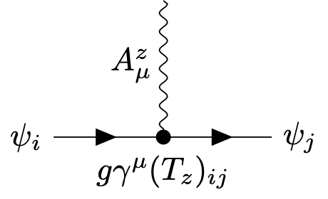
similar to the vertex \(e \gamma^\mu\) for photons.

Neutron decay

An example in the electroweak \(\text{SU}(2)\) theory is

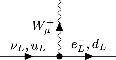
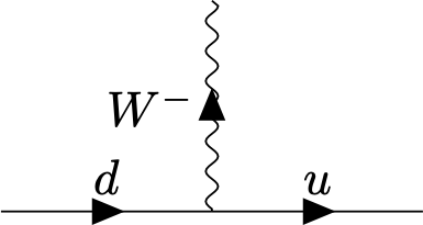
The fermion species can be changed in the vertex due to \((T_z)_{ij}\) ! This leads to interesting effects, such as the decay of the neutron, \[n\to p^++e^-+\bar\nu,\] The quark decomposition of the neutron \(n\) is \(udd\) and of the proton \(p\) it is \(uud\). The electric charge of \(u\) is \(2/3\) and of \(d\) is \(-1/3\). Out of the vertex

and

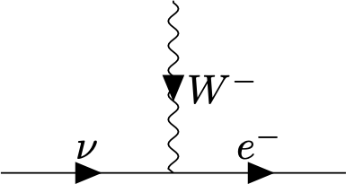
one can construct a neutron decay process

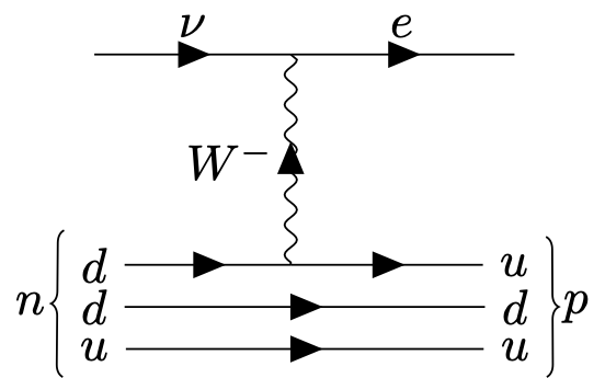
For small momenta, the \(W\)-propagator can be approximated by \(\eta^{\mu\nu}/m_W^2\). This leads to the pointlike four-fermion interaction of the form \[\frac{g^2}{m_W^2} \left[\bar u_L(x) \gamma^\mu d_L(x)\right] \left[\bar e_L(x)\gamma_\mu\nu_L(x)\right].\] Such effective vertices are known from Fermis theory of weak interactions. The mass of the \(W\) boson \(m_W^2 \sim g^2 \phi_0^2\) is generated by the Higgs mechanism, and accordingly the strength of the four-fermion vertex in Fermis theory is proportional to \(1/\phi_0^2\). This allows a rough estimate of the Higgs field expectation value \(\phi_0\).

Self interactions

There is a crucial difference between non-Abelian and Abelian gauge theories. For an Abelian gauge theory, the photon has no self-interaction since it is neutral. As a consequence, Maxwell’s equations are linear.

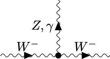
In contrast, for non-Abelian gauge theories such as Yang-Mills theories, there is a self-interaction between gluons. The gluons carry color charge, not only the quarks. The field equations thus become non-linear. The necessity for interaction with gauge bosons is also clear for the \(W^\pm\)-bosons. In particular they are charged and interact with the photon.

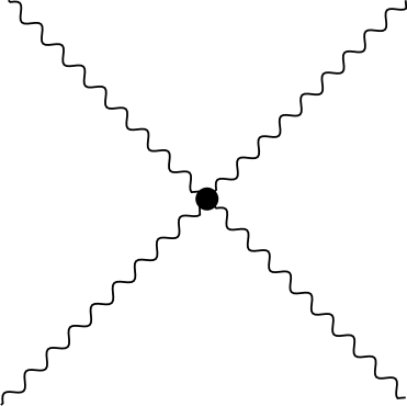
We next need a gauge covariant kinetic term which generalizes the Maxwell action for the photon. It is given in Minkowski space conventions by \[S_\text{Yang-Mills} = \int_x \left\{ - \frac{1}{4} F_z^{\mu\nu}(x)F_{\mu\nu}^z(x) \right\} = \int_x \left\{ - \frac{1}{2 g^2} \text{tr}\left\{\mathbf{F}^{\mu\nu}\mathbf{F}_{\mu\nu}\right\} \right\}.\] Here we recall that the field strength is given by \[F^z_{\mu\nu}(x) = \partial_\mu A_\nu^z(x)-\partial_\nu A_\mu^z(x) + g f_{yw}^{~~z} A_\mu^y(x) A_\nu^w(x).\] The action \(S_\text{Yang-Mills}\) contains terms with three gluons leading to a vertex

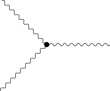
and with four gluon fields, leading to a vertex

Similarly, in the electroweak theory one has interaction vertices of the form

Let us note here that the Yang-Mills action is actually by itself a non-trivial theory for interacting gauge fields. We will see later that it becomes strongly interacting in the infrared, and it is not easily solved.

Action for spinor gauge theory

We now have all the components to construct an action for a gauge theory with fermions and gauge bosons. We just need to combine the part for Dirac fermions with the kinetic part for gauge fields, \[\begin{split} S = & S_\text{Dirac}+S_\text{Yang-Mills} \\ = & \int_x \left\{ - \bar \psi(x) \gamma^\mu \left[\partial_\mu - i \mathbf{A}_\mu(x)\right] \psi(x) - \frac{1}{2g^2} \text{tr}\left\{ \mathbf{F}^{\mu\nu}(x) \mathbf{F}_{\mu\nu}(x) \right\} \right\} \\ = & \int_x \left\{ - \bar \psi(x) \gamma^\mu \left[\partial_\mu - i g A^z_\mu(x)T_z \right] \psi(x) - \frac{1}{4} F^{z \mu\nu}(x) F^z_{\mu\nu}(x) \right\}. \end{split}\] This is the basic structure of quantum chromodynamics (QCD), but also of the fermionic and gauge field sector of the electroweak theory.

Problems with gauge freedom

When one attempts to derive a propagator for the Yang-Mills gauge fields, one encounters the same problems as for the photon. In fact, at quadratic level in the gauge field the self-interaction drops out, and Yang-Mills fields are like a collection of several copies of the photon. Recall that an inverse photon propagator is proportional to \(p^2 \delta^\mu_{~\nu} - p^\mu p_\nu = p^2 \mathscr{P}^\mu_{~\nu}\), and it is not invertible. In fact, this matrix has a vanishing eigenvalue corresponding to the eigenvector \(p^\mu\). This problem is a direct consequence of the gauge freedom.

To understand this in more detail, let us decompose the (Abelian) gauge field into a longitudinal or pure gauge part \(A^L_\mu(x) = \partial_\mu \beta(x)\), and a remainder term \(A^T_\mu(x)\), \[A_\mu(x) = \partial_\mu\beta(x) + A^T_\mu(x).\] This decomposition becomes unique when \(A^T_\mu(x)\) is fixed to obey a specific gauge condition, such as the Landau gauge \(\partial^\mu A^T_\mu(x)=0\). The QED action is invariant under \(A_\mu(x)\to A_\mu(x) + \partial_\mu \alpha(x)\) or \(\beta(x)\to \beta(x)+\alpha(x)\). This means that it does not depend on the longitudinal part \(A^L_\mu(x)=\partial_\mu\beta(x)\). Accordingy, fluctuations of \(A^L_\mu(x)=\partial_\mu\beta(x)\) are not suppressed in the functional integral and contribute an infinite factor. At the same time, physical observables should be gauge invariant and not depend on \(A^L_\mu(x)\).