
Quantum field theory 2, lecture 08
One loop effective potential for three spatial dimensions
The computations for the classical statistics in three dimensions are similar. One now has \[\Delta m^2= \frac{3 \bar{\lambda}_\Lambda}{8 \pi^2} \int_0^{\Lambda^2}dx x^{\frac{1}{2}} \frac{1}{x+\bar m^2_\Lambda}\] and \[\Delta \lambda= -\frac{9 \bar{\lambda}_\Lambda^2}{8 \pi^2} \int_0^{\Lambda^2}dx x^{\frac{1}{2}} \frac{1}{(x+\bar m^2_\Lambda)^2}.\] Inspecting the momentum integrals, one finds that \(\Delta m^2 \sim \Lambda\) is UV-dominated, while \(\Delta \lambda\) is now IR-dominated! One finds \[\Delta \lambda= - \frac{9 \bar{\lambda}_\Lambda^2}{16 \pi^2} \frac{1}{\sqrt{\bar m^2_\Lambda} }\] For \(\bar{m}_\Lambda\to 0\) one observes an IR-divergence for \(\Delta \lambda\). This is a major difficulty for perturbative calculations for \(d=3\) near phase transitions!
Perturbative renormalization
So far we have parametrized our theory in terms of the microscopic parameters \(\bar m^2_\Lambda\) and \(\bar\lambda_\Lambda\). But these are not quantities that are easily accessible to any experiment. The strategy is therefore to replace these microscopic parameters by macroscopic quantities \(m^2\) and \(\lambda\). The microscopic or “bare” parameters \(\bar m^2_\Lambda\) and \(\bar{\lambda}_\Lambda\) are not known. In contrast, the renormalized parameters \(m^2\) and \(\lambda\) can be determined by measurements; for example they enter directly in the computation of propagators, cross sections etc.
Within perturbation theory, one expands in the small renormalized coupling \(\lambda\). We concentrate here on the leading terms in \(\lambda\) or \(\bar \lambda_\Lambda\). Moreover, let us concentrate here on \(d=4\) dimensions.
Mass renormalization
The full or renormalized mass is at one-loop order given by \[m^2 =\bar m^2_\Lambda + \frac{3 \bar{\lambda}_\Lambda}{32 \pi^2} \Lambda^2 - \frac{3 \bar{\lambda}_\Lambda}{32 \pi^2} \ln\left(\frac{\Lambda^2+\bar m^2_\Lambda}{\bar m^2_\Lambda}\right).\] This implies that one can express to leading order in the coupling \(\lambda\) the microscopic or bare mass parameter as \[\bar m^2_\Lambda = m^2 - \frac{3 \lambda}{32 \pi^2}\Lambda^2 + \frac{3 \lambda}{32 \pi^2}\ln\left(\frac{\Lambda^2+m^2}{m^2}\right)+\mathcal{O}(\lambda^2).\]
Coupling renormalization
The full quartic coupling constant is to leading order \[\lambda = \bar{\lambda}_\Lambda - \frac{9 \bar{\lambda}_\Lambda^2}{32 \pi^2}\left( \ln \frac{\Lambda^2+\bar m^2_\Lambda}{\bar m^2_\Lambda}-1 \right) \approx \bar{\lambda}_\Lambda \left( 1 - \frac{9}{32 \pi^2}\lambda \ln \frac{\Lambda^2}{m^2} \right)\] This allows to express the microphysics or bare couling constant as \[\bar{\lambda}_\Lambda = \frac{\lambda}{1 - \frac{9}{32 \pi^2}\lambda \ln\left(\frac{\Lambda^2}{m^2}\right)}.\] For fixed \(\lambda\) the bare quartic coupling \(\bar{\lambda}_\Lambda\) diverges at a “Landau pole" when \(\ln(\Lambda^2/m^2)= 32 \pi^2/(9 \lambda)\). This indicates a limit of validity of the theory. Arbitrary high \(\Lambda\) are not possible for given \(\lambda\) !
In the opposite direction for fixed \(\lambda_\Lambda\), \(\Lambda\) and \(m^2\rightarrow 0\) one has \(\lambda\rightarrow 0\). This phenomenon is known as “triviality of \(\Phi^4\) theory". For a given finite \(\Lambda\) one finds an upper bound for \(\lambda\) and therefore the mass of the Higgs boson in the standard model. For \(\Lambda\) in the region of a few TeV the resulting bound is \(m_\text{Higgs} \lesssim 500\, \text{GeV}\).
Sextic coupling
The \(\Phi^6\) coupling \(\gamma= 27 \lambda^3/(32 \pi^2m^2)\) is fixed in terms of \(\lambda\) and \(m^2\). There is no additional free parameter. The theory is specified in terms of only two renormalized parameters, \(m^2\) and \(\lambda\).
Momentum dependence of \(\Phi^4\)-vertex
The one-particle irreducible four point vertex depends on the momentum of of the incoming or outgoing particles \[\Gamma^{(4)}(p_1,p_2,p_3,p_4) = 3 \tilde{\lambda}(p_1,p_2,p_3) (2\pi^4)\delta^{(d)}(p_1+p_2-p_3-p_4)\] The Feynman graph for the fluctuation contribution is given by
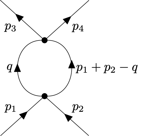
In this notation, the quartic coupling \(\lambda\) computed previously corresponds to \(\tilde{\lambda}(0,0,0)=\lambda\). The difference \[\lambda(p_1,p_2,p_3)-\lambda(0,0,0),\] is then found to be IR-dominated. It does not depend on \(\Lambda\). In perturbation theory it is computable and found \(\sim \lambda^2\). Cutoff corrections are \(\sim 1/\Lambda^2\) and vanish for \(\Lambda\to \infty\). The difference is therefore predictable! The whole momentum dependence of \(\Gamma^{(4)}\) and the associated cross sections are predicted in terms of the two parameters \(\lambda\) and \(m^2\).
The lesson we learn here is that IR-dominated quantities are predictable! Only a finite number of renormalized couplings needs to be specified! The same strategy works actually for QED, with the renormalized coupling being the electric charge \(e\) in addition to the particles masses.
Renormalizable theories miracle
Once all quantities are expressed in terms of renormalized couplings, all momentum integrals become ultraviolet finite for \(\Lambda\to \infty\), even for higher loops. Theories with this property are called renormalizable theories. For renormalizable theories, the limit \(\Lambda \to \infty\) can be taken! This works very similar in other regularizations schemes, e. g. in the limit \(d \to 4\) within dimensional regularizaton.
Typical renormalized parameters are \(m^2\) and \(\lambda\) for \(\phi^4\) theory, \(m_e\) and \(e\) for QED and the quark mass \(m_q\) and the strong couling constant \(g_s\) for QCD. All other quantities are then predictable in terms of these.
Predictivity and irrelevant operators
IR-dominated terms in the quantum effective action \(\Gamma[\Phi]\) are known as “irrelevant operators”. Key elements for the predictability of QFT in situations where microphysics is not precisely known are
symmetries
fluctuation domination of “irrelevant operators”
Additional predictivity arises in situations where further microphysics is actualy known.
Example in QED, anomalous magnetic momentum of muon
As an example for the principles discussed above, let us take the magnetic moment of the electron, or muon. First, the Dirac theory without radiative corrections gives the magentic moment in Bohr units \[g=2.\] Quantum corrections yield corrections to this result such that \(g-2 \neq 0\).
Specifically, a quantum vertex from the diagram
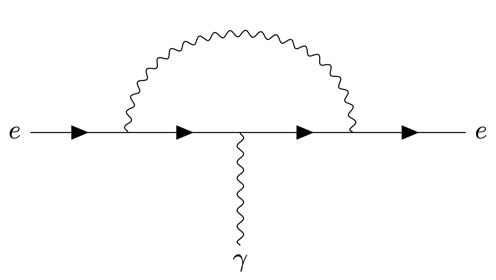
leading to a term of the form \[\Delta\Gamma = \int_x \left\{c\, \bar{\psi}(x) [\gamma^\mu, \gamma^\nu] \psi(x) F_{\mu\nu}(x) \right\}.\] Such a term is consistent with all all symmetries. The dimension of \(c\) is \(\text{mass}^{-1}\), and in an unknown misroscopic theory defined at a scale \(\Lambda\) one would expect \(c\) to be of order \(1 /\Lambda\).
Quantum corrections to \(c\) are IR-dominated, with leading cutoff dependent terms proportional to \(1 /\Lambda\). As a consequence, for large scale separation, \(\Lambda\to \infty\), the correction \(g-2\) becomes predictable! For pure QED (with loops involving electrons, muons, taons and photons) this calculation has been done for the muon anomaleous magnetic moment in perturbation theory up to five loops1, \[\begin{split} \left[\frac{g-2}{2}\right]_\text{QED} = \frac{\alpha}{2\pi} & + 0.765 857 420(13) \left(\frac{\alpha}{\pi}\right)^2 + 24.050 509 85(23) \left(\frac{\alpha}{\pi}\right)^3 \\ & + 130.8782(60) \left(\frac{\alpha}{\pi}\right)^4 + 751.0(9) \left(\frac{\alpha}{\pi}\right)^5 + \ldots \end{split}\] The leading term is the classical one-loop result obtained by Schwinger, and will be recalculated as an excercise. With the experimental value for the inverse of the electromagnetic fine structure constant \(1/\alpha = 137.035 999 046(27)\) one finds \[\left[\frac{g-2}{2}\right]_\text{QED} = 0.00116 584 718 93(10).\] The latest experimental result based on experiments at Brookhaven National Lab and at Fermilab is2 \[\left[\frac{g-2}{2}\right]_\text{experiment} = 0.00116592061(41).\] The difference is \[7342(41) \times 10^{-11},\] and pure QED (without hadrons) is excluded at more that \(100 \sigma\) level.
Electroweak fluctuation effects (\(W^{\pm}\) bosons, \(Z\) bosons and Higgs bosons) also contribute to \(g-2\), and have been calculated to two-loop order plus leading three-loop terms, \[\Delta \left[\frac{g-2}{2}\right]_\text{electroweak} = 154(1) \times 10^{-11}.\] Most difficult are calculations of the hadronic contribution to \(g-2\). A recent lattice-QCD simulation gave3 \[\Delta \left[\frac{g-2}{2}\right]_\text{hadronic} = 7075(55) \times 10^{-11}.\] With this, there is currently not a big discrepancy between theory and experiment. The hardronic theory calculation is to be confirmed by other groups.
Gauge theories
Local transformations
Gauge theories are models with a local symmetry. For the example of complex fermionic or scalar fields \(\psi(x)\) one has \[\begin{split} \psi(x)\to U(x)\psi(x). \end{split}\] An important example are the strong interactions which are described by the gauge group \(\text{SU}(3)\). Here the fields \(\psi(x)\) are for quarks (up, down, strange, charm, bottom or top) that are each in a color-triplet. In other words, \(\psi\) is a complex three component Grassmann field, and \(U\) a matrix \[\psi_j(x), \quad\quad\quad U_{ij}(x),\] such that the transformation law becomes \[\psi_i(x) \to \psi_i^\prime(x)=U_{ij}(x)\psi_j(x),\] where \(i,j = 1,\ldots,3\) are the color indices.
The color group SU\((3)\)
The transformation matrices \(U(x)\) are elements of the group SU\((3)\) of special unitary transformation in three complex dimensions, \[U^\dagger U=\mathbb{1},\quad\quad\quad \text{det}(U)=1.\] The group structure is obvious, with the unit matrix being the unit element, inverse \(U^{-1}=U^\dagger\), the composition law \(U_1U_2=U_3\), such that with \(U_3^\dagger= (U_1U_2)^\dagger= U_2^\dagger U_1^\dagger\) one has \(U_3^\dagger U_3=U_2^\dagger U_1^\dagger U_1 U_2 = \mathbb{1}\), and \(\det(U_3)= \det(U_1)\det(U_2)= 1\). Also associativity is clear, \(U_1(U_2U_3)=(U_1U_2)U_3\). The composition is non-Abelian, however, \(U_1 U_2 \neq U_2 U_1\).
The weak group SU\((2)\)
Similarly, the weak interactions involve an SU\((2)\)-gauge symmetry, for which left-handed leptons and quarks are doublets, i. e. two-component complex Grassmann fields \[\begin{split} \begin{pmatrix} \nu(x)\\ e(x) \end{pmatrix}_L,\quad\quad\quad \begin{pmatrix} u_i(x)\\ d_i(x) \end{pmatrix}_L, \end{split}\] and so on. The left-handed part of a Dirac field is obtained with the projection \[\begin{split} \psi_L(x) = P_L \psi(x) = \frac{1}{2}(\mathbb{1}+\gamma_5)\psi(x). \end{split}\] In this case, \(U(x)\) is a complex \(2\times 2\)-matrix. For the standard model, one has an additional Abelian U\((1)\) symmetry under which left- and right-handed fermions transform with different charges.
Lie groups and exponential map
Lie groups are continuous groups which are also differentiable manifolds.4 They have the interesting property that they can be characterized by the transformations that are infinitesimally close to the unit element, in terms of the Lie algebra.
Finite group transformations can be composed of many small ones with the exponential map \[U = \lim_{N\to\infty} \left( \mathbb{1} + \frac{i\alpha^z T_z}{N}\right)^N = \exp\left(i\alpha^zT_z \right).\] Here \(\alpha^z T_z\) (with summation over the index \(z\) implied) is an element of the Lie algebra, and the \(T_z\) are the generators of the Lie algebra. The coefficients are real, \(\alpha^z \in \mathbb{R}\).
One distinguishes between the abstract Lie group and a representation of it. As for any group, a representation has the same composition laws as the abstract group itself. With a representation of the group comes a representation of its algebra and vice versa.
Infinitesimal transformations
Because finite transformations can be composed out of many ininitesimal ones, it is for many applications sufficient to consider infinitesimal transformations. These are very close to the unit element, \[U = \mathbb{1} + i\alpha^z T_z,\] in the sense that \(\alpha^z\) is infinitesimal. Fields in the fundamental representation transform under an infinitesimal gauge transformation according to \[\psi(x) \to \psi(x)+\delta\psi(x) = \psi(x) + i\alpha^z(x) T_z \psi(x).\]
R.L. Workman et al. (Particle Data Group), Prog. Theor. Exp. Phys. 2022, 083C01 (2022).↩︎
B. Abi et al. (Muon g-2 Collaboration) Phys. Rev. Lett. 126, 141801 (2021).↩︎
Borsanyi, S., Fodor, Z., Guenther, J.N. et al., Nature 593, 51–55 (2021).↩︎
For an introduction to Lie groups and Lie algebras in physics, see also the course “Symmetries” https://www.tpi.uni-jena.de/~floerchinger/teaching/↩︎