Quantum field theory 2, lecture 07

Full coupling constants and one-loop contributions

We consider a polynomial expansion of \(U(\rho)\), with \(U^\prime(\rho)= \partial U(\rho)/\partial\rho\), and so on, and define the full coupling constants based on the effective potential, \[\begin{split} m^2 = & U^\prime(0) = \bar{m}^2_\Lambda+U_\text{1-loop}^\prime(0),\\ \lambda = & U^{\prime\prime}(0) = \bar{\lambda}_\Lambda+U_\text{1-loop}^{\prime\prime}(0),\\ \gamma = & U^{(3)}(0)=U_\text{1-loop}^{(3)}(0). \end{split}\] The first two decompose into a microscopic part and a one-loop contribution. Note that \(\gamma\) is a six-point vertex not present in the classical actions. This is a “quantum vertex”.

Feynman graphs

We want to evaluate \[\begin{split} \Delta m^2 = & \frac{\partial}{\partial \rho}U_\text{1-loop}(\rho) \\ = & \frac{3 \bar{\lambda}_\Lambda}{2}\int_p \frac{1}{p^{2}+\bar{m}^2_\Lambda+3 \bar{\lambda}_\Lambda \rho }. \end{split}\] This corresponds to a one-loop Feynman diagram

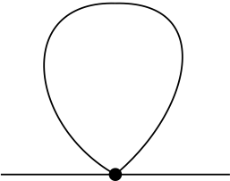
Lines are given by the classical propagator \(G=(P^2+\bar{m}_\Lambda^2+3\bar{\lambda}_{\Lambda}\rho)^{-1}\), and the point denotes the classical vertex \(\partial^{4}V/\partial \phi^{4} = 3 \bar{\lambda}_\Lambda\). As usual, a closed line involves a trace, i.e. a momentum integral and a sum over contracted indices.

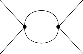
In a similar way we obtain higher order derivatives, \[\frac{\partial^2}{\partial \rho^2} U_\text{1-loop}(\rho) = -\frac{9 \bar{\lambda}^2_\Lambda}{2} \int_p \frac{1}{(p^2+\bar{m}^2_\Lambda+3 \bar{\lambda}_\Lambda \rho)^2},\] with Feynman diagram

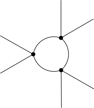
and \[\frac{\partial^3}{\partial \rho^3} U_\text{1-loop}(\rho) = 27\bar{\lambda}^3_\Lambda \int_p \frac{1}{(p^2+\bar{m}^2_\Lambda+3 \bar{\lambda}_\Lambda \rho)^3},\] with Feynman diagram

Evaluating these expressions at \(\rho=0\), we find the one-loop corrections \[\begin{split} \Delta m^2&= \frac{3 \bar{\lambda}_\Lambda}{2}\int_p \frac{1}{p^2+\bar{m}_\Lambda^2},\\ \Delta \lambda&=- \frac{9 \bar{\lambda}_\Lambda^2}{2}\int_p \frac{1}{(p^2+\bar{m}_\Lambda^2)^2},\\ \Delta \gamma &=27\bar{\lambda}_\Lambda^3\int_p \frac{1}{(p^2+\bar{m}_\Lambda^2)^3}. \end{split}\] We recall here the abbreviation \[\int_p = \int \frac{d^d p}{(2\pi)^d}.\]

Regularization

Some of the expressions we encounter here show divergent behaviour in the high momentum or ultraviolet regime of the momentum integrals. These need to be regularized by imposing a suitable cutoff at a scale \(\Lambda\). Ultimately we would like to take the limit where the ultraviolet regulator becomes largem, \(\Lambda \to \infty\). Also, there could be additional infrared divergences from the lower limit of the momentum integral. In Euclidean space this is not the case for \(m_\Lambda^2>0\).

For the UV-regularization one has different possibilities, and they have different advantages and disadvantages. Let us start by stating a few general properties of the integrals involved. For the effective potential we are concerned with integrals of the form \[\begin{split} \int \frac{d^d p}{(2\pi)^d} f(p^2) = & \frac{\Omega_d}{(2\pi)^d} \int_0^\infty dp \, p^{d-1} f(p^2) \\ = & \frac{\Omega_d}{2 (2\pi)^d} \int_0^\infty dx \, x^{(d-2)/2} f(x) \end{split}\] Here we use the surface are of the unit sphere in \(d\) dimensions \[\Omega_d = \frac{2 \pi^{d/2}}{\Gamma(d/2)}.\] Well known special values are \(\Omega_1=2\), \(\Omega_2=2\pi\), \(\Omega_3=4\pi\) and \(\Omega_4=2\pi^2\). However, it is often useful to keep \(d\) open, not only because one can then specialize to different physics models, but also because a non-integer value of \(d\) provides a possible regularization scheme by itself (dimensional regularization).

Sharp UV cutoff

A simple possibility to regularize the one-loop integrals in the UV is to impose a sharp cutoff by restricting the integrals to \(p^2=x < \Lambda^2\). Let us now also specialize to \(d=4\).

One-loop contribution to mass squared

For the loop correction to the mass term, we need the integral \[\begin{split} \int_p \frac{1}{p^2+\bar{m}_\Lambda^2}&=\frac{1}{16\pi^2}\int_0^{\Lambda^2}dx \frac{x}{x+\bar{m}_\Lambda^2}= \frac{1}{16 \pi^2}\left[ \Lambda^2-\int_0^{\Lambda^2}dx \frac{\bar{m}_\Lambda^2}{x+\bar{m}_\Lambda^2} \right] \\ &=\frac{1}{16\pi^2}\left[ \Lambda^2- \bar{m}^2_\Lambda \ln\left(\frac{\Lambda^2+\bar{m}_\Lambda^2}{\bar{m}_\Lambda^2}\right)\right], \end{split}\] resulting in \[\begin{split} \Delta m^2&=\frac{3 \bar{\lambda}_\Lambda}{32\pi^2}\left[ \Lambda^2- \bar{m}^2_\Lambda \ln\left( \frac{\Lambda^2+\bar{m}_\Lambda^2}{\bar{m}_\Lambda^2}\right)\right]. \end{split}\] One concludes that bosonic fluctuations increase the mass term! The loop contribution to the mass squared would have a leading quadratic divergence with the regulator scale \(\Lambda\) in the limit \(\Lambda\to\infty\).

In the standard model, one has \(m\approx 100\,\text{GeV}\), while grand unification or gravity scales are \(\Lambda\approx 10^{15}\,\text{GeV}\) and \(\Lambda\approx 10^{18}\,\text{GeV}\) respectively. With \[m^2=\bar m^2_\Lambda +g^2 \Lambda^2,\] a small mass does not seem natural.

One-loop contribution to quartic coupling

For the quartic coupling we can use a simple identity \[\begin{split} \int_p \frac{1}{(p^2+\bar{m}_\Lambda^2)^2}&=-\frac{\partial}{\partial \bar{m}_\Lambda^2}\int_p \frac{1}{p^2+\bar{m}_\Lambda^2}\\ & = \frac{1}{16\pi^2}\left[ \ln\left(\frac{\Lambda^2+\bar m^2_\Lambda}{\bar m^2_\Lambda}\right)+\bar m^2_\Lambda \frac{\partial}{\partial \bar m^2_\Lambda}\ln\left( \frac{\Lambda^2+\bar m^2_\Lambda}{\bar m^2_\Lambda} \right) \right] \\ & = \frac{1}{16\pi^2}\left[ \ln\left( \frac{\Lambda^2+\bar m^2_\Lambda}{\bar m^2_\Lambda}\right)+ \frac{\bar m^2_\Lambda}{\Lambda^2+\bar m^2_\Lambda}-1 \right]. \end{split}\] Neglecting terms \(\sim 1/\Lambda^{n}\) with \(n>0\) yields \[\int_p \frac{1}{(p^2+\bar{m}_\Lambda^2)^2} = \frac{1}{16\pi^2}\left[ \ln\left( \frac{\Lambda^2}{\bar m^2_\Lambda}\right)-1 \right],\] which implies the one-loop contribution to the quartic coupling \[\Delta \lambda =- \frac{9 \bar{\lambda}_\Lambda^2}{32 \pi^2}\left[ \ln\left(\frac{\Lambda^2}{\bar{m}_\Lambda^2}\right)-1 \right].\] The interaction strength is driven to smaller values by the loop corrections. Now the dependence on the regulator scale is only logarithmic.

One-loop contribution to sextic coupling

Finally we consider the loop contribution to the quantum vertex \(\gamma\). Here we can use our previous result with the calculational trick \[\begin{split} \int_p \frac{1}{(p^2+\bar{m}_\Lambda^2)^3} = & -\frac{1}{2} \frac{\partial}{\partial \bar m^2_\Lambda}\int_p \frac{1}{(p^2+\bar m^2_\Lambda)^2} \\ = & \frac{1}{32 \pi^2 \bar m^2_\Lambda}. \end{split}\] The last line is the leading expression for \(\Lambda\to\infty\) and it is actually finite! Accordingly we find the one-loop contribution to the six-point vertex \[\gamma = \frac{27 \lambda_\Lambda^3}{32 \pi^2} \frac{1}{\bar{m}_\Lambda^2}.\]

Fluctuation effects

The one-loop corrections increase the mass, reduce the 4-vertex coupling strength and generates new 6-point vertex, \[m^2>\bar m^2_\Lambda,\quad\quad\quad \lambda<\bar{\lambda}_\Lambda,\quad\quad\quad \gamma> \gamma_\Lambda=0.\] Note that \(\Delta m^2\sim \Lambda^2\) and \(\Delta\lambda\sim-\ln(\Lambda^2/\bar m^2_\Lambda)\) are divergent for \(\Lambda\to \infty\), while \(\gamma\) becomes independent of the regulator scale. There is an interesting relation to the canonical mass dimension here. Obviously \(m^2\) has dimensions of mass squared, \(\lambda\) is dimensionless in four dimensions, and \(\gamma\) has dimensions of inverse mass squared.

Separation of scales

Typically one has a separation between large momentum scales of order \(\Lambda\) and much smaller scales of order \(\bar m_\Lambda\) or \(m\). This assumes small coupling \(\lambda_\Lambda\ll 1\). One can infer that different quantities are dominated by rather different momentum ranges in the loop integral:

• The mass squared correction \(\Delta m^2\) is dominated by modes \(p^2\approx \Lambda^2\). It is UV-dominated, i. e. by microscopic physics.

• The correction to the quartic interaction \(\Delta \lambda\) is logarithmically divergent for \(\Lambda\rightarrow\infty\). All momentum modes contribute here.

• The sextic coupling \(\gamma\) is independent of \(\Lambda\). It is dominated by modes with \(p^2\approx \bar m^2_\Lambda\), or IR-dominated, and independent of microscopic physics.

Impact of fluctuation effects on mass term

Since the mass correction is positive, \(\Delta m^2>0\), it is possible to have a negative bare mass term \(\bar m^2_\Lambda<0\) but a positive renormalized mass term \(m^2>0\). Then the system is in the symmetric phase, even for \(\bar m^2_\Lambda<0\). This happens for Ising type models. One has local order but not global order. Strong fluctuation effects destroy the order!

In thermal equilibrium for \(T\neq0\) the fluctuation correction \(\Delta m^2\) depends on \(T\). This can lead to a phase transition as a function of temperature. The fluctuation contribution \(\Delta m^2(T)\) is monotonically increasing with \(T\).

The phase transition occurs at \(T_c\). At the critical temperature the mass term vanishes \(m^2(T_c)=0\). For fermions the sign of the fluctuation effects is opposite. The contribution from fermion fluctuations amounts to \(\Delta m^2<0\). For the standard model this may lead to top-quark induced electroweak symmetry breaking.

Predictivity of QFT

The sextic vertex \(\gamma\) can be predicted! One may add to the microscopic model a \(\phi^6\) coupling. By dimension counting it is of the form \(\bar{\gamma}_\Lambda\sim 1/\Lambda^2\). The macroscopic coupling \(\gamma\) is dominated by the fluctuation contribution, and an additional microscopic coupling \(\bar{\gamma}_\Lambda\) plays no role for \(\Lambda\to\infty\).

In other words, we may add to the classical potential a term \[V_6 = \frac{1}{48} \frac{\tilde \gamma}{\Lambda^2}\varphi^6,\] with dimensionless coupling \(\tilde \gamma\). This yields for the ratio of the fluctuation contribution and the classical contribution \[\frac{\text{fluctuation contribution}}{\text{classical contribution}}= \frac{27 \bar{\lambda}_\Lambda^3}{32 \pi^2} \frac{6}{\tilde \gamma} \frac{\Lambda^2}{\bar{m}^2}.\] One infers that the fluctuation contribution dominates for large ratio \(\Lambda /\bar{m}\).