Quantum field theory 2, lecture 26

Field theoretic discussion

Let us now investigate the response function from a quantum field theory point of view. We can write the expectation value as a functional integral along a Schwinger-Keldysh path from some initial time \(t_\text{in}<y^0\) forwards, until the time \(x^0\) (or later) then backwards to the initial time \(t_\text{in}\), and then downwards in the complex time plane to the point \(t_\text{in} - i \beta\) where the countour is closed.

This corresponds to \[\langle \chi_a(x) \rangle = \frac{1}{Z}\int D\phi_+ D\phi_-D\phi_0 \left\{ \chi_a(x) e^{iS_\text{M}[\phi_+]} e^{-S_\text{E}[\phi_0]} e^{-iS_\text{M}^*[\phi_-]} \right\},\] where \(S_\text{M}[\phi_+]\) is a Minkoski space action for forward time evolution with the usual \(i\epsilon\) terms, \(S_\text{M}^*[\phi_-]\) its relative for backward time evolution where the sign if the \(i\epsilon\) terms is reversed, and \(S_\text{E}[\phi_0]\) is a Euclidean action that describes the thermal density matrix at time \(t_0\) in the Matsubara formalism.

The functional integrals have to be clued with the following boundary conditions at the initial time \(t_0\) \[\phi_+(t_0, \mathbf{x}) = \phi_0(t_0-i\beta, \mathbf{x}), \quad\quad\quad \phi_-(t_0, \mathbf{x}) = \phi_0(t_0, \mathbf{x}),\] and at the time \(t_\text{f} = x^0\) (or any time later that that) one must set \[\phi_+(t_\text{f}, \mathbf{x}) = \phi_-(t_\text{f}, \mathbf{x}).\] Taking now into account that \[S[\phi] = S_0[\phi] + \int d^dy \left\{ j_b(y) \chi_b(y)[\phi] \right\}\] leads to a contribution from the expansion of the forward evolving action \(S_\text{M}[\phi_+]\) proportional to \(i \langle \chi_a(x) \chi_b(y) \rangle\) and one from the backward evolving action. Using the cyclic property of the trace it can be understood as \(-i\langle \chi_b(y) \chi_a(x) \rangle\). Both contributions vanish for \(y^0 > x^0\) by causality, or formally because the correspnding parts of the forward and backward evolution operators cancel. In summary we find \[\Delta_{ab}(x-y) = i \theta(x^0-y^0) \langle \left[ \chi_a(x) , \chi_b(y) \right] \rangle = \Delta^R_{ab}(x-y).\] This is simply the retarded correlation function we have discussed previously! In other words, linear response experiments can directly access the retarded two-point correlation between the responding field \(\chi_a(x)\) and the perturbation field \(\chi_b(y)\) to which the source \(j_b(y)\) couples.

Static and dynamic susceptibilities

Consider a source function of the form \[j_b(t^\prime,\mathbf{y}) = \theta(-t^\prime) e^{\epsilon t^\prime} %\int \frac{d^{d-1} p}{(2\pi)^{d-1}} e^{i\mathbf{p}\mathbf{y}} j_b(0,\mathbf{y}).\] It grows very slowely or “adiabatically” in time, until it is switched off at time \(t^\prime=0\). The response is given by \[\begin{split} \bar \chi_a(t,\mathbf{x}) = & \int_{-\infty}^0 dt^\prime \int \frac{d\omega}{2\pi} \int \frac{d^{d-1}p}{(2\pi)^{d-1}} e^{-i\omega(t-t^\prime)+\epsilon t^\prime + i \mathbf{p}(\mathbf{x}-\mathbf{y})} \Delta^R_{ab}(\omega, \mathbf{p}) j_b(0,\mathbf{y}) \\ = & \int \frac{d\omega}{2\pi i} \int \frac{d^{d-1}p}{(2\pi)^{d-1}} e^{-i\omega t + i \mathbf{p}(\mathbf{x}-\mathbf{y})} \frac{1}{\omega -i\epsilon} \Delta^R_{ab}(\omega, \mathbf{p}) j_b(0,\mathbf{y}). \end{split}\] Setting now also \(t=0\), the \(\omega\) integration can be closed in the upper half of the complex plane. There is only a single pole at \(\omega=i\epsilon\) because \(\Delta^R_{ab}(\omega, \mathbf{p})\) must be analytic in the upper half plane for causality. Accordingly one finds (taking now \(\epsilon\to 0\)) \[\bar \chi_a(0, \mathbf{x}) = \int \frac{d^{d-1}p}{(2\pi)^{d-1}} e^{i \mathbf{p}(\mathbf{x}-\mathbf{y})} \Delta^R_{ab}(0, \mathbf{p}) j_b(0,\mathbf{y}).\] This response can similarly be written in terms of the advanced Greens function, and we have previously seen that the difference between retarded and advanced Green functions, wich is the spectral density, must vanish for \(\omega\to 0\).

The function \[\chi_{ab}(\mathbf{p}) = \Delta^R_{ab}(0, \mathbf{p}) = \Delta^A_{ab}(0, \mathbf{p}),\] is a static linear response function also known as static susceptibility. It can be determined directly in thermal equilibrium and describes the reponse of a thermal expectation value to a change in the Hamiltonian.

In contrast to this, the response function \(\Delta^R_{ab}(\omega, \mathbf{p})\) at non-vanishing frequency \(\omega\) contains information about the relaxation to equilibrium, or about thermalization dynamics, and needs a real time calculation or analytic continuation. It is also known as dynamic susceptibility.

Static and dynamic structure factors

Let us consider now the statistical correlation function for bosonic fields \[\Delta^S_{ab}(x-y) = \frac{1}{2} \langle \chi_a(x) \chi_b(y) + \chi_b(y) \chi_a(x) \rangle = \int_ p e^{ip(x-y)} \Delta^S_{ab}(p).\] For commuting fields (no canonical conjugate momentum fields involved) this is simply the correlation function \(\langle\chi_a(x) \chi_b(x) \rangle\). When the times agree, \(x^0=y^0\), this gives the equal-time correlation function, \[\Delta^S_{ab}(0, \mathbf{x}-\mathbf{y}) = \int \frac{d^{d-1}p}{(2\pi)^{d-1}} e^{i\mathbf{p}(\mathbf{x}-\mathbf{y})} S_{ab}(\mathbf{p}),\] with the frequency integral \[S_{ab}(\mathbf{p}) = \int \frac{d\omega}{2\pi} \Delta^S_{ab}(\omega, \mathbf{p}),\] also known as the static structure factor. It can be experimentally accessed by recording values of the field \(\chi_a(t, \mathbf{x})\) as a function of spatial position \(\mathbf{x}\) (and the discrete index \(a\) when applicable), instanteneously at some time \(t\). This is like “taking pictures”. From many such recordings one can construct correlation functions. Similar to the static susceptibility, the equal-time correlation function or the static structure factor are thermal equilibrium properties and can be calculated in the Matsubara formalism without analytic continuation.

In contrast, the more general object \(S_{ab}(\omega, \mathbf{p})=\Delta_{ab}^S(\omega, \mathbf{p})\) is known as dynamic structure factor. Experimentally it can be accessed by inelastic scattering spectroscopy with the elastic limit corresponding to \(\omega=0\). Its Fourier transform, the statistical or structure correlation function \(\Delta^S_{ab}(x^0 - y^0, \mathbf{x}-\mathbf{y})\) is also known as van Hove coorelation function.

Self energy loop diagram

We now consider a frequency and momentum dependent loop diagram in a finite temperature situation, and allow also for chemical potential terms. The diagram involves two propagators, and it appears in this or a related form in many circumstances, for example as a correction to the inverse propagator when there are three point vertices, or as a subdiagram of a vertex correction.

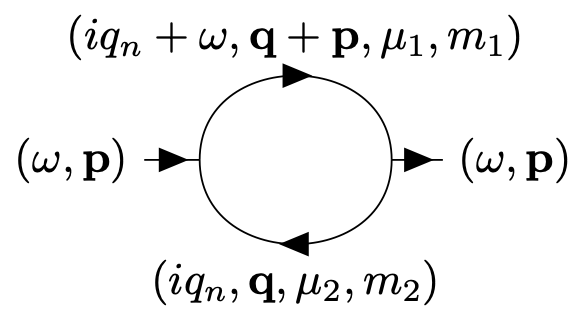
We take the incoming frequency and momentum to be \((\omega, \mathbf{p})\) where \(\omega\) is a real frequency which we should consider to be analytically continued from a Matsubara feequency \(\omega=i 2\pi T m\). To cover the general case, we allow the two propagators in the loop to have chemical potentials \(\mu_1\) and \(\mu_2\), and masses \(m_1\) and \(m_2\), respectively.

We find for the core of the diagram \[S(\omega, \mathbf{p}) = - T \sum_{n=-\infty}^\infty \int_\mathbf{q} \frac{1}{\left[-(iq_n+\omega + \mu_1)^2 + (\mathbf{q}+\mathbf{p})^2 + m_1^2\right]\left[-(iq_n+ \mu_2)^2 + \mathbf{q}^2 + m_2^2\right]}.\] The minus sign has been added because it will typically appear like this in a concrete application, e. g. in perturbation theory.

Matsubara propagators in time domain

The Matsubara propagators appearing here can be written in the form \[\frac{1}{(q_n-i\mu)^2+\mathbf{q}^2+m^2} = \int_{0}^{\beta} d\tau e^{iq_n \tau} J(\tau, \mu, \sqrt{\mathbf{q}^2+m^2}).\] This uses the Matsubara sum we have calculated previously \[\begin{split} J(\Delta\tau, \mu, x) = & T\sum_{n=-\infty}^\infty \frac{e^{-i2\pi T n \Delta\tau}}{(2\pi T n -i\mu)^2+x^2} \\ = & \frac{1}{2x} \left[ \theta(\Delta\tau) + n_B(x-\mu) \right] e^{-(x-\mu)\Delta\tau} + \frac{1}{2x} [\theta(-\Delta\tau) + n_B(x+\mu)] e^{(x+\mu)\Delta\tau} \\ = & \sum_{s=\pm 1} \frac{s}{2x} \left[ \theta(\Delta\tau) + n_B(s x-\mu) \right] e^{-(sx-\mu)\Delta\tau} \end{split},\] as well as the identity \[T \int_{0}^{\beta} d\tau e^{i2\pi T n\tau} = \delta_{0n}.\] Note that the precise integration bounds are somewhat arbitrary here, and one could equally well integrate from some point \(\sigma\) to \(\sigma+\beta\). The symmetric choice we made simplifies some of the following steps.

We find thus \[\begin{split} S(\omega, \mathbf{p}) = & - T \sum_{n=-\infty}^\infty \int_\mathbf{q} \int_{0}^{\beta} d\tau_1 d\tau_2 \, e^{iq_n(\tau_1+\tau_2)+\omega\tau_1} \\ & \times J{\Big (}\tau_1, \mu_1, \sqrt{(\mathbf{q}+\mathbf{p})^2 + m_1^2} {\Big )} J{\Big (}\tau_2, \mu_2, \sqrt{\mathbf{q}^2 + m_2^2}{\Big )}. \end{split}\]

Peforming sums and integrals

At this point one can perform the sum over \(n\) using \[T \sum_{n=-\infty}^\infty e^{i 2\pi T n (\tau_1+\tau_2)} = \sum_{k=-\infty}^\infty \delta(\tau_1+\tau_2-k \beta).\] For our choice of integration interval for Matsubara frequencies only one Dirac delta with \(k=1\) actually contributes. Using this one can perform one of the time integrals, resulting in \[\begin{split} S(\omega, \mathbf{p}) = & - \int_\mathbf{q} \int_{0}^{\beta} d\tau \, e^{\omega\tau} J{\Big (}\tau, \mu_1, \sqrt{(\mathbf{q}+\mathbf{p})^2 + m_1^2} {\Big )} J{\Big (}\beta-\tau, \mu_2, \sqrt{\mathbf{q}^2 + m_2^2}{\Big )}. \end{split}\] Using the concrete expression for \(J\) one can now perform also the integral over the remaining Matsubara time \(\tau\). One finds integrals of the form \[\begin{split} \int_{0}^{\beta} d\tau \exp(\omega\tau+x_1\tau+x_2(\beta-\tau)) = & \frac{\exp((\omega+x_1)/T) - \exp(x_2/T)}{\omega+x_1-x_2} \\ \to & \frac{\exp(x_1/T) - \exp(x_2/T)}{\omega+x_1-x_2}, \end{split}\] where \(x_1\) and \(x_2\) are combinations of energies and chemical potentials. In going from the first to the second line we have used that \(\omega\) is analytically continued from points on the Matsubara axis where \(\omega=i 2 \pi T m\). On all these points one has \(\exp(\omega/T) = 1\).

Proceeding this way gives with \(E_1=\sqrt{(\mathbf{q}+\mathbf{p})^2 + m_1^2}\) and \(E_2=\sqrt{\mathbf{q}^2 + m_2^2}\) \[\begin{split} S(\omega, \mathbf{p}) = - \int_{\mathbf{q}} \frac{1}{4E_1E_2} & \left\{ % \frac{ [1+n_B(E_1-\mu_1)] [1+n_B(E_2-\mu_2)] \left[\exp(-\frac{E_1-\mu_1}{T}) - \exp(-\frac{E_2-\mu_2}{T})\right] }{ \omega - E_1+\mu_1 + E_2-\mu_2 } \right. \\ % & \quad + \frac{ [1+n_B(E_1-\mu_1)] n_B(E_2+\mu_2) \left[\exp(-\frac{E_1-\mu_1}{T}) - \exp(\frac{E_2+\mu_2}{T})\right] }{ \omega - E_1+\mu_1 - E_2+\mu_2 } \\ % & \quad + \frac{ n_B(E_1+\mu_1) [1+n_B(E_2-\mu_2)] \left[\exp(\frac{E_1+\mu_1}{T}) - \exp(-\frac{E_2-\mu_2}{T})\right] }{ \omega + E_1+\mu_1 + E_2-\mu_2 } \\ % & \left. \quad + \frac{ n_B(E_1+\mu_1) n_B(E_2+\mu_2) \left[\exp(\frac{E_1+\mu_1}{T}) - \exp(\frac{E_2+\mu_2}{T})\right] }{ \omega + E_1+\mu_1 - E_2-\mu_2 } % \right\}. \end{split}\] Here one can use the identities \[\exp(z/T) n_B(z) = 1+n_B(z),\] and \[\exp(-z/T) [1+n_B(z)] = n_B(z).\]

Interpreting the branch cut through loss minus gain

Combining terms we find \[\begin{split} S(\omega, \mathbf{p}) = \int_{\mathbf{q}} \frac{1}{4E_1E_2} & \left\{ % \frac{ [1+n_B(E_1-\mu_1)] [1 + n_B(E_2+\mu_2)] - n_B(E_1-\mu_1) n_B(E_2+\mu_2) }{ \omega - E_1+\mu_1 - E_2-\mu_2 } \right. \\ & \quad + \frac{ n_B(E_1+\mu_1) n_B(E_2-\mu_2) - [1+ n_B(E_1+\mu_1)][1 + n_B(E_2-\mu_2)] }{ \omega + E_1+\mu_1 + E_2-\mu_2 } \\ % & \quad + \frac{ [1+ n_B(E_1-\mu_1)] n_B(E_2-\mu_2) - n_B(E_1-\mu_1) [1+n_B(E_2-\mu_2) ] }{ \omega - E_1+\mu_1 + E_2-\mu_2 } \\ & \left. \quad + \frac{ n_B(E_1+\mu_1) [1+ n_B(E_2+\mu_2)] - [1+n_B(E_1+\mu_1)] n_B(E_2+\mu_2) }{ \omega + E_1+\mu_1 - E_2-\mu_2 } % \right\}. \end{split}\] This can be simplified further, but as it stands the different terms have a very nice physical interpretation.

Specifically, the branch cut part of \(S(\omega, \mathbf{p})\) is obtained by replacing \[\frac{1}{\omega-E_1+\mu_1-E_2-\mu_2} \to -i \pi \, s_\text{I}(\omega) \, \delta(\omega - E_1+\mu_1 - E_2-\mu_2),\] and so on. It is indeed on the real frequency axis. The resulting Dirac delta implies energy conservation. The physical interpretation of the imaginary part is a difference between loss and gain processes.

Specifically, the term in the first line describes the transition from the incoming state with frequency \(\omega\) into a two-particle state with energy \(E_1+E_2\) minus the transition from such a two-particle state into the outgoing state. For the decay parts one has Bose enhancement of the vaccum amplitudes when the modes are already occupied. The gain process comes from thermally occupied modes.

Similarly, the second line describes a transition of the incoming particle with energy \(\omega\) together with two anti-particles from the bath into an empty state minus the gain process which is a decay into two anti-particles and the outgoing state.

The third line describes a reaction of the incoming particle with frequeny \(\omega\) together with an anti-particle with energy \(E_2\) into a particle with energy \(E_1\) minus the corresponding gain term.

Finally, the last line stands for a reaction of the incoming particle with an anti-particle of energy \(E_1\) into a particle of energy \(E_2\) minus the gain term.

We observe that the entire brach cut part of \(S(\omega, \mathbf{p})\) can be written as loss minus gain, where the ratio of loss over gain is \(\exp(\omega/T)\), following detailed balance.

Vacuum self energy and decay rate

In the vaccum limit \(T=\mu_1=\mu_2=0\) one finds \[S(\omega, \mathbf{p}) = \int_{\mathbf{q}} \frac{1}{4E_1E_2} \left\{ % \frac{ 1 }{ \omega - E_1 - E_2 } - \frac{ 1 }{ \omega + E_1 + E_2 } \right\}.\] Assuming now \(m_1=m_2=m\), the brach cut starts here at \(\omega^2 - \mathbf{p}^2 = 4m^2\) or for \(\mathbf{p}=0\) at \(|\omega| = 2 m\), which corresponds to the energy threshold for the production of two particles with mass \(m\). It is simplest to calculate this for \(\omega>0\), \(\mathbf{p}=0\) where \(E_1=E_2=\sqrt{\mathbf{q}^2+m^2}\). Evaluating the integrand for \(\text{Im}(\omega) = \pm \epsilon\) gives for the branch cut part of \(S(\omega,\mathbf{p})\) \[\text{Disc } S(\omega, \mathbf{p}) = -i \pi s_\text{I}(\omega) \int_{\mathbf{q}} \frac{1}{4E^2} [\delta(\omega - 2E) - \delta(\omega + 2E)].\] The remaining integral can be done using the Dirac delta. It is an integral over the phase space for the decay into the two particles. Using that the result must be Lorentz invariant gives \[-i \pi s(\omega) \theta(\omega^2-\mathbf{p^2}-4m^2) \frac{\Omega_{d-1}}{(2\pi)^{d-1}2^{d}} \frac{(\omega^2-\mathbf{p}^2-4m^2)^\frac{d-2}{2}}{\sqrt{\omega^2-\mathbf{p}^2}},\] with \[s(\omega) = \text{sign}(\text{Im}(\omega)) \, \text{sign}(\text{Re}(\omega)).\] This is the imaginary part that corresponds to the continuum of two-particle states. It could also been calculated with the help of Cutkosky cutting rules. We see here a manifestation of the optical theorem, telling that the imaginary part of the forward amplitude must be propational to the decay propability into a continuum of scattering states!

Vanishing chemical potentials but finite temperature

At vanishing chemical potentials \(\mu_1=\mu_2=0\) we obtain for the branch cut \[\begin{split} \text{Disc }S(\omega, \mathbf{p}) = -i s_\text{I}(\omega) \pi \int_{\mathbf{q}} \frac{1}{4E_1E_2} {\Big \{ } & % \left[ [1+n_B(E_1)] [1 + n_B(E_2)] - n_B(E_1) n_B(E_2) \right] \delta(\omega - E_1 - E_2) \\ + & \left[ n_B(E_1) n_B(E_2) - [1+ n_B(E_1)][1 + n_B(E_2)]\right] \delta( \omega + E_1 + E_2) \\ % + & \left[ [1+ n_B(E_1)] n_B(E_2) - n_B(E_1) [1+n_B(E_2) ] \right] \delta( \omega - E_1 + E_2 ) \\ + & \left[ n_B(E_1) [1+ n_B(E_2)] - [1+n_B(E_1)] n_B(E_2)\right] \delta(\omega + E_1 - E_2 ) % {\Big \} }. \end{split}\] As mentioned before, all terms decompose naturally into a loss minus a gain term which differ by a factor \(\exp(\omega/T)\). This allows to write \[\text{Disc }S(\omega, \mathbf{p}) = -i s_\text{I}(\omega) \pi \left[ e^{\frac{\omega}{2T}} - e^{-\frac{\omega}{2T}} \right]\left[ H(\omega, \mathbf{p}) + H(-\omega, \mathbf{p}) \right]\] where \[\begin{split} H(\omega, \mathbf{p}) = \int_{\mathbf{q}} \frac{1}{4E_1E_2} % \left[ n_B(E_1) e^{\frac{E_1}{2T}} n_B(E_2) e^{\frac{E_2}{2T}} \right] [\delta(\omega - E_1 - E_2) + \delta(\omega-E_1+E_2)] . \end{split}\]