Quantum field theory 2, lecture 24

Observables at equal and un-equal times

With the thermal equilibrium formalism one can directly calculate observables such as expectation values or correlation functions on a single Cauchy hypersurface \(\Sigma\), for example at some time \(t_0\). Formally this is done by finding the corresponding operator \(A_\Sigma[\phi_1, \phi_2]\) and its expectation value \[\langle A \rangle = \text{Tr} \left\{ \rho A_\Sigma \right\} = \int D\phi D\phi^\prime \rho[\phi,\phi^\prime] A_\Sigma[\phi^\prime, \phi].\] For a global equilibrium state, the state is actually time translation invariant in the direction of the Killing vector field \(\beta^\mu(x)\), so the hypersurface \(\Sigma\) could be placed at different times.

In addition to this, it is also possible to calculate expectation values and correlation functions at different times. For this, one needed to supplement the operators with pieces for time evolution - forwards and backwards. This leads to a functional integral with braches for forward and backward time evolution, the Schwinger-Keldysh double time path, and it is also the idea underlying the Heisenberg picture of quantum theory, which we shall use in the following.

Linear response theory

Two-point function for thermal equilibrium states

We will now discuss two-point correlation functions for a quantum field theory in thermal equilibrium. We work here in Minkowski space with cartesian coordinates where \(\beta^\mu(x) = \beta^\mu\) is constant. One can also find a Lorentz frame, the fluid rest frame, where \(\beta^\mu = (1/T,0,0,0)\), but we largely keep the frame general.

Let us start from the correlation function of two fields \(\chi_a(x)\) and \(\chi_b(y)\) which might be elementary fields but could as well be composite operators such as pairing fields or for example energy density, particle density or similar, \[\Delta_{ab}^+(x-y) = \langle \chi_a(x) \chi_b(y) \rangle = \text{tr} \left\{ \rho \, \chi_a(x) \chi_b(y) \right\} .\] We can allow \(\chi_a(x)\) and \(\chi_b(x)\) to be both bosonic or fermionic. The mixed case can be excluded because a mixed correlation function needs to vanish. The indices \(a\) and \(b\) are also used to label representations of the Lorentz group. For example they could label spinor components for the Dirac field of vector components for currents etc.

Note that the fields are not necessarily time-ordered here. When \(x\) and \(y\) are at different times, we need to insert convenient time evolution operators to evaluate the trace on the Cauchy surface where \(\rho\) is defined. We use here the notation of the operator formalism, but one could of course work in a functional representation.

We take the density matrix to correspond to a thermal equilibrium with temperature \(T\) and fluid velocity \(u^\mu\) (a possible chemical potential can be included as an external gauge field), \[\rho = \frac{1}{Z} \exp\left(P_\mu \beta^\mu \right),\] where \(P^\mu=(H, \mathbf{P})\) is a four-momentum operator, which we could write as a Cauchy surface integral involving the energy-momentum tensor.

The fields \(\chi_a(x)\) and \(\chi_b(y)\) have the Heisenberg representation \[\chi(x) = \exp(-iP_\mu x^\mu ) \chi(0) \exp(i P_\mu x^\mu),\] which also involves the four-momentum operator.

Using complete basis of momentum eigenstates

Introduce now a complete set of states which are eigenstates of the four-momentum operator, \[P^\mu | m \rangle = p^\mu_m |m \rangle.\] The energies are non-negative, \(p^0\geq 0\). The normalization is taken to be such that \[\mathbb{1} = \sum_m | m \rangle \langle m |, \quad\quad\quad \langle m | n \rangle = \delta_{mn} .\] The thermal density matrix becomes \[\rho = \frac{1}{Z}\sum_m e^{p_m\beta} | m \rangle \langle m |.\] For simplicity, we use a notation as for discrete states, but in reality there will also be a continuum of states \(|m\rangle\). One obtains \[\begin{split} \Delta_{ab}^+(x-y) = & \sum_{m,l}\frac{1}{Z} e^{p_m\beta} \langle m | e^{-iP x} \chi_a(0) e^{iPx} |l\rangle \langle l | e^{-iPy} \chi_b(0) e^{iPy} |m \rangle \\ = & \sum_{m,l} \frac{1}{Z} e^{p_m\beta} e^{i (p_l - p_m)(x-y)} \langle m | \chi_a(0) | l \rangle \langle l | \chi_b(0) | m \rangle . \end{split}\] We introduce also the momentum space representation \[\Delta^+_{ab}(x-y) = \int \frac{d^4 p}{(2\pi)^4} e^{ip(x-y)} \; \Delta^+_{ab}(p) ,\] and find by Fourier transform \[\Delta_{ab}^+(p) = \sum_{m,l} \delta^{(4)}(p-p_l+p_m) \frac{1}{Z} e^{p_m \beta} \langle m | \chi_a(0) | l \rangle \langle l | \chi_b(0) | m \rangle .\] One can see this as the probability amplitude for the process \[p_m \overset{\chi_b}{\longrightarrow} p_m + p \overset{\chi_a}{\longrightarrow} p_m.\] Starting from a state with thermal occupation and energy-momentum \(p_m\), \(\chi_b(0)\) mediates a transition to a state with energy \(p_l=p_m+p\) and \(\chi_a(0)\) mediates a transition back to the original state.

Positive and negative energies

The sum over \(m\) contains a Boltzmann weight where energies that are large compared to the temperature are exponentially suppressed. For \(T \to 0\) only the ground state with \(p_m=0\) survives in the sum over \(m\) and one has \[\Delta_{ab}^+(p) =\sum_l \delta^{(4)}(p-p_l) \langle 0 | \chi_a(0) | l \rangle \langle l | \chi_b(0) | 0 \rangle \quad\quad\quad\quad\quad (\text{for }T \to 0). % %\label{eq:TzeroLimit}\] One observes that there is only a contribution with \(p\neq 0\) when \(\chi_b(0)\) creates an excitation with momentum \(p\) which is subsequently destroyed by \(\chi_a(0)\). The energy \(p_0\) must be above the energy of the vacuum state and accordingly \(\Delta_{ab}^+(p)\) only has support for \(p^0\geq 0\) and it is then a transition amplitude. This is the reason for labeling it with a plus.

For non-vanishing temperature, the part of \(\Delta_{ab}^+(p)\) at negative frequency \(p^0<0\) corresponds to a transition from a positive energy state with thermal occupation to one with smaller energy induced by \(\chi_b(0)\) before the energy is recovered again through \(\chi_a(0)\).

Reversed argument correlation function and detailed balance

Using analogous steps, the correlation function with reversed field arguments, \[\Delta_{ba}^+(y-x) = \langle \chi_b(y) \chi_a(x) \rangle = \int \frac{d^4 p}{(2\pi)^4} e^{ip(x-y)} \Delta_{ba}^+(-p),\] can be written as \[\Delta_{ba}^+(-p) = \sum_{m,l} \delta^{(4)}(p-p_m+p_l) \frac{1}{Z} e^{p_m \beta} \langle m | \chi_b(0) | l \rangle \langle l | \chi_a(0) | m \rangle.\] One can see this as the probability amplitude for the process \[p_m \overset{\chi_a}{\longrightarrow} p_m - p \overset{\chi_b}{\longrightarrow} p_m.\] Starting from a state with thermal occupation and energy-momentum \(p_m\), \(\chi_a(0)\) mediates a transition to a state with energy \(p_l=p_m-p\) and \(\chi_b(0)\) mediates a transition back to the original state. This is the reverse process to the oe described by \(\Delta_{ab}^+(p)\). In thermal equilibrium there must be detailed balance between all the intermediate processes. In other words, the rates, which are transition probabilities or squared transition amplitudes times Boltzmann weights, for forward and backward processes, must be equal. This intuitively explains the identity \[\Delta_{ba}^+(-p) = \exp(p\beta) \Delta_{ab}^+(p),\] which can be derived easily from the explicit expressions.

Spectral and statistical correlation functions

Define now also the spectral and statistical correlation functions by \[\begin{split} \Delta^\rho_{ab}(x-y) = & \langle \left[\chi_a(x), \chi_b(y) \right]_\mp \rangle = \text{tr} \left\{ \rho \left[\chi_a(x), \chi_b(y)\right]_\mp \right\} = \int_p e^{ip(x-y)} \Delta^\rho_{ab}(p), \\ % \Delta^S_{ab}(x-y) = &\frac{1}{2} \langle \left[\chi_a(x), \chi_b(y) \right]_\pm \rangle = \frac{1}{2} \text{tr} \left\{ \rho \left[\chi_a(x), \chi_b(y)\right]_\pm \right\} = \int_p e^{ip(x-y)} \Delta^S_{ab}(p). \end{split} \label{eq:defDeltaRhoDeltaS}\] For bosonic fields the spectral function \(\rho_{ab}\) involves the commutator (upper sign), for fermionic fields the anti-commutator (lower sign). For the statistical propagator it is the opposite.

Intuitively, the statistical correlation function carries information about fluctuations, for example it could be evaluated at equal time to yield the correlation function in the thermal equilibrium state. In contrast, the spectral function contains information about propgation in time and response to perturbations (see below).

One can express the spectral correlation function in terms of \(\Delta^+_{ab}(p)\), \[\Delta^\rho_{ab}(p) = \Delta_{ab}^+(p) \mp \Delta_{ba}^+(-p) = \left( 1 \mp \exp(p \beta) \right) \Delta_{ab}^+(p) ,\] and similarly the statistical correlation function, \[\Delta^S_{ab}(p) = \frac{1}{2} \left[\Delta_{ab}^+(p) \pm \Delta_{ba}^+(-p) \right] = \frac{1}{2} \left( 1 \pm \exp(p \beta) \right) \Delta_{ab}^+(p).\]

Fluctuation-dissipation relation

Comparing the two expressions for the spectral and statistical functions yields the important fluctuation-dissipation relation (H. B. Callen and T. A. Welton, 1951) \[\Delta^S_{ab}(p) = \left[ \frac{1}{2} \pm n_{B/F}(\omega) \right] \Delta^\rho_{ab}(p) , \label{eq:FluctDissRelation}\] where \(\omega = - u_\mu p^\mu\) is the frequency in the fluid rest frame, and the Bose and Fermi occupation number functions introduced previously \[n_{B/F}(\omega) = \frac{1}{e^{\omega/T}\mp 1}.\] Note that the square bracket in the fluctuation dissipation relation is anti-symmetric under \(p^\nu \to - p^\nu\), as was shown previously.

The fluctuation-dissipation theorem holds in thermal equilibrium only, and it corresponds to the statement of detailed balance between forward and backward processes. More generally, the statistical and spectral correlation functions are not related in a simple way. In the vacuum state at zero temperature only the quantum fluctuations survive, corresponding to the term \(1/2\) in the square bracket. In the high-temperature or classical limit, the square bracket becomes in the bosonic case \(T/\omega\).

From the definitions one can also obtain the expression for the spectral function \[\Delta^\rho_{ab}(p) = \sum_{m,l} \delta^{(4)}(p-p_l+p_m) \frac{1}{Z} \left(e^{p_m \beta} \mp e^{p_l\beta} \right) \langle m | \chi_a(0) | l \rangle \langle l | \chi_b(0) | m \rangle.\] For the statistical correlation function one has a similar expression, but with an additional factor \(1/2\) and the opposite sign between the two Boltzmann weights in the round bracket. For bosonic fields this implies that the spectral function must vanish, \(\Delta^\rho_{ab}(p)\to 0\), in the zero frequency limit \(p\beta\to 0\), because the Dirac distribution implies \(p_l\beta=p_m\beta\) then. For fermionic fields a similar statement holds for the statistical correlation function \(\Delta^S_{ab}(p)\).

More Greens functions

It is useful to define also the Feynman, retarded and advanced propagators through the equations \[\begin{split} -i \Delta^F_{ab}(x-y) = & \langle T \, \chi_a(x) \chi_b(y) \rangle = \theta(x^0-y^0) \langle \chi_a(x) \chi_b(y) \rangle \pm \theta(y^0-x^0) \langle \chi_b(y) \chi_a(x) \rangle , \\ % -i \Delta^R_{ab}(x-y) = & \theta(x^0 - y^0) \langle \left[ \chi_a(x) , \chi_b(y)\right]_\mp \rangle , \\ % -i \Delta^A_{ab}(x-y) = & - \theta(y^0 - x^0) \langle \left[ \chi_a(x) , \chi_b(y)\right]_\mp \rangle , \end{split} \label{eq:DefFeynmanRetardedAdvanced}\] with corresponding momentum space representations \(\Delta^F_{ab}(p)\), \(\Delta^R_{ab}(p)\) and \(\Delta^A_{ab}(p)\). Typically these are Greens functions to some inverse propagator which is a combination of derivative operators, and they differ through their boundary conditions. While the Feynman propagator is time-ordered, the retarded propagator is only non-vanishing for \(x^0>y^0\) and the advanced propagator for \(y^0> x^0\).

From the Feynman propagator one obtains via analytic continuation through Wick rotation of the frequency axis the Matsubara propagator. In momentum space, and for simplicity in the fluid rest frame, \[\begin{split} & \Delta^M(i \omega_n, \mathbf{p}) = \Delta^F(\omega = i \omega_n , \mathbf{p}) . \end{split}\]

Useful relations

The following relations between retarded and advanced functions follow directly from the definitions \[\Delta^R_{ab}(x-y) = \pm\Delta^A_{ba}(y-x), \quad\quad\quad \Delta^A_{ab}(x-y) = \pm \Delta^R_{ba}(y-x) ,\] or, in momentum space, \[\Delta^R_{ab}(p) = \pm \Delta^A_{ba}(-p), \quad\quad\quad \Delta^A_{ab}(p) = \pm \Delta^R_{ba}(-p) .\] If one known the retarded function one also knows the advanced one, and vice versa.

The spectral correlation function can be written in terms of the difference of retarded and advanced Greens functions, \[\Delta^\rho_{ab}(p) = -i \Delta^R_{ab}(p) + i \Delta^A_{ab}(p) , \label{eq:rhoRA}\] an identity that also follows directly from the definitions. Finally, the statistical correlation function can be obtained from this via the fluctuation-dissipation relation.

Complex argument Greens function and spectral representation

For simplicity we specialize now to the fluid rest frame. For homogeneous equilibrium states (which includes the vacuum as a special case), the spectral function \(\Delta^\rho_{ab}(\omega, \mathbf{p})\) plays a special role. It determines all other correlation functions through an integral representation.

We define the complex argument Greens function by the integral over the spectral function \[G_{ab}(\omega, \mathbf{p}) = \int_{- \infty}^\infty \frac{dz}{2\pi} \; \Delta^\rho_{ab}(z, \mathbf{p}) \frac{1}{z-\omega}. %\label{eq:GSpectralRep}\] The integral over \(z\) is along the real axis.

The function \(G_{ab}(\omega, \mathbf{p})\) can be evaluated for complex frequency argument \(\omega \in \mathbb{C}\). It has a brach cut or poles along the real \(\omega\) axis, but, importantly, nowhere else! This follows from the integral relation above, which is known as the spectral representation.

One can show that one obtains the Feynman, retarded, advanced and Matsubara Greens functions by evaluating \(G\) on the contours close to the real \(\omega\) axis, but shifted slightly away it.

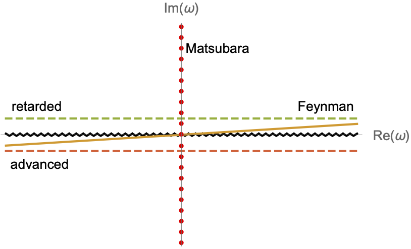
Specifically, the retarded Greens function is obtained by evaluating \(G_{ab}(\omega, \mathbf{p})\) slightly above the real frequency axis. It has then by construction on poles or brach cuts in the upper half of the complex frequency plane, which leads to the right causality structure when one goes back to real space. Similarly the advanced Greens function is obtained by evaluating \(G_{ab}(\omega, \mathbf{p})\) slightly below the real frequency axis, and the Feynman propagator by evaluating \(G_{ab}(\omega, \mathbf{p})\) below the real frequency argument when \(\text{Re}(\omega)\) is negative, and above it when \(\text{Re}(\omega)\) is positive. This is equivalent to the usual \(i\epsilon\) prescription.

In terms of formula, \[\begin{split} \Delta^R_{ab}(p) = & G_{ab}\left(\omega + i \epsilon, \mathbf{p} \right) , \\ \Delta^A_{ab}(p) = & G_{ab}\left(\omega - i \epsilon, \mathbf{p} \right) , \\ \Delta^F_{ab}(p) = & G_{ab}\left(\omega + i \epsilon\; \text{sign}(\omega), \mathbf{p} \right) , \\ \Delta^M_{ab}(p) = & G_{ab}\left(i \omega_n , \mathbf{p} \right) . \end{split} %\label{eq:RetAdvFeynMatFromCompArgGreensFunc}\]

Using the identity \[\frac{1}{x\pm i\epsilon} = \mp i \pi \delta(x) + \text{P.V. } \frac{1}{x},\] where the second term is the Cauchy principal value, one can see that the difference between retarded and advanced Greens functions leads indeed back to the spectral density.