
Quantum field theory 2, lecture 22
Contour integral around imaginary axis
In order to find a way to sum over \(n\), we first consider a complex contour integral \[J = \frac{1}{2\pi i} \int_{\mathcal{C}} dz \left\{ \frac{e^{-z\Delta\tau}}{-( z+\mu)^2+x^2}\left[ \theta(\Delta\tau) + n_B(z) \right] \right\}.\] Here, \(\mu\) and \(x\geq 0\) as well as \(\Delta\tau\) with \(-1/T < \Delta\tau < 1/T\) are parameters. The integration contour \(\mathcal{C}\) goes downwards slightly left of the imaginary \(z\)-axis and up again slightly to the right of it.
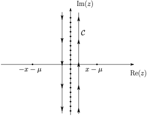
We use here the Bose distribution function \[n_B(z) = \frac{1}{e^{z/T}-1},\] which has poles at \(z=i2\pi T n\) for all integer \(n\in \mathbb{Z}\), with residue \(T\). It is also useful to keep in mind that for positive argument \(z>0\) one has the zero temperature limit \[\lim_{T\to 0} n_B(z) = 0.\] Similarly, in the high-temperature limit one has \[\lim_{T\to\infty} n_B(z) = \frac{T}{z}.\]
The term \(-(z+\mu)^2+x^2\) has zero-crossings at \[\begin{split} z = \pm x - \mu. \end{split}\] We assume \(|\mu|<x\), so that those poles stay away from the imaginary \(z\)-axis. The contour can be closed at \(z=\pm i\infty\) and we find from the residue theorem \[J = T\sum_{n=-\infty}^\infty \frac{e^{-i 2\pi T n \Delta\tau}}{(2\pi n T -i\mu)^2+x^2}.\] This is precisely the infinite sum we need to calculate!
Contour integral around real axes
On the other side, wen can also close the contour somewhat differently without changing the result.
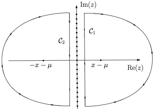
We now get two contributions, \(J=J_1+J_2\), one contour \(\mathcal{C}_1\) that closes on the right and one contour \(\mathcal{C}_2\) that closes on the left. From \[\frac{1}{-(z+\mu)^2+x^2} = \left( - \frac{1}{z-x+\mu} + \frac{1}{z+x+\mu} \right) \frac{1}{2x}\] one can read off where the poles are. Closing the contour \(\mathcal{C}_1\) at large positive real values of \(z\) is unproblematic when \(0\leq \Delta\tau <\beta\), because \(e^{-z\Delta\tau}\) decays quickly. However, also when \(-\beta < \Delta\tau \leq 0\) this is fine because the constant part in \(\theta(\Delta\tau) + n_B(z)\) is then absent and \(n_B(z)\) decays asymptotically more quickly than \(e^{-z\Delta\tau}\) grows. Taking into account that the contour has now a clockwise orientation gives a contribution from \(\mathcal{C}_1\) \[J_1 = \frac{1}{2x} \left[ \theta(\Delta\tau)+ n_B(x-\mu) \right] e^{-(x-\mu)\Delta\tau}.\] On the other side, closing the contour \(\mathcal{C}_2\) at large negative real \(z\) is also possible, because one can use the identity \[1+n_B(z) + n_B(-z) = 0,\] to replace \(\theta(\Delta\tau)+n_B(z)\) by \(-[\theta(-\Delta\tau)+n_B(-z)]\) and then use similar arguments as for \(J_1\). We find thus a contribution from \(\mathcal{C}_2\) \[J_2 = \frac{1}{2x} [\theta(-\Delta\tau) + n_B(x+\mu)] e^{(x+\mu)\Delta\tau}.\] In summary, from the different possibilities to perform the contour integration, \(J=J_1+J_2\), we obtain the formula \[\begin{split} T\sum_{n=-\infty}^\infty \frac{e^{-i2\pi T n \Delta\tau}}{(2\pi T n -i\mu)^2+x^2} = & \frac{1}{2x} \left[ \theta(\Delta\tau) + n_B(x-\mu) \right] e^{-(x-\mu)\Delta\tau} \\ & + \frac{1}{2x} [\theta(-\Delta\tau) + n_B(x+\mu)] e^{(x+\mu)\Delta\tau}. \end{split}\] This identity allows to calculate the Matsubara sums for bosons! It also gives the right result for \(T\to 0\) as one may check by a direct integration. In that limit the terms proprtional to \(n_B\) simply drop out. Similar techniques involving contour integrals can be used also for the Matsubara sums appearing in perturbative diagrams or renormalization group flow equations at finite temperature.
Result for scalar boson propagator
We can now combine terms and find for the boson propagator on the Matsubara torus \[\begin{split} \Delta(\Delta\tau, \Delta\mathbf{x}) = \int_\mathbf{p} \frac{e^{i\mathbf{p}\mathbf{x}}}{\sqrt{\mathbf{p}^2+m^2}} & \left( \left[ \theta(\Delta\tau)+n_B(\sqrt{\mathbf{p}^2+m^2}-\mu) \right] e^{-(\sqrt{\mathbf{p}^2+m^2}-\mu)\Delta\tau} \right. \\ & \left. + \left[\theta(-\Delta\tau) + n_B(\sqrt{\mathbf{p}^2+m^2}+\mu)\right] e^{(\sqrt{\mathbf{p}^2+m^2}+\mu)\Delta\tau} \right). \end{split}\]
Contour integral around imaginary axis for fermions
For fermionic Matsubara sums we need to go through similar steps. Let us start with the contour integral \[K = \frac{1}{2\pi i} \int_{\mathcal{C}} dz \left\{ \frac{e^{-z\Delta\tau}}{-( z+\mu)^2+x^2}\left[ \theta(\Delta\tau) - n_F(z) \right] \right\}.\] The integration contour goes again up slightlt to the right of the imaginary \(z\) axis, and down slightly to the left of it.
We use the Fermi distribution function \[n_F(z) = \frac{1}{e^{z/T}+1}.\] The latter has poles at \(z=i 2\pi T (n+\frac{1}{2})\) with residue \(-T\). Closing the contour at \(z=i \pm \infty\) and using the residue theorem gives \[K = T\sum_{n=-\infty}^\infty \frac{e^{-i 2\pi T (n+\frac{1}{2}) \Delta\tau}}{(2\pi (n+\frac{1}{2}) T -i\mu)^2+x^2}.\] This is a typical Matsubara sum appearing when working with fermions.
Contour integral around real axes for fermions
Again one can alternatively close the contour integrals around the real \(z\) axes. Many arguments are similar as in the bosonic case. A noteable difference is that we should not assume \(|\mu|<x\) because this would not allow a Fermi sphere which builds up at small temperature. However, because there is no Matsubara frequency with \(\omega_n=0\), it is possible to deform the integration contours such that it goes through between the two poles in the decomposition \[\frac{1}{-(z+\mu)^2+x^2} = \left( - \frac{1}{z-x+\mu} + \frac{1}{z+x+\mu} \right) \frac{1}{2x}.\] Proceeding carefully gives from \(\mathcal{C}_1\) the contribution \[K_1 = \frac{1}{2x} [\theta(\Delta\tau) - n_F(x-\mu)] e^{-(x-\mu)\Delta\tau}.\] Similarly, from \(\mathcal{C}_2\) we obtain \[K_2 = \frac{1}{2x} [\theta(-\Delta\tau) - n_F(x+\mu)] e^{(x+\mu)\Delta\tau}.\] In summary, using \(K=K_1+K_2\) we find a pocket formula for ferminic Matsubara sums \[\begin{split} T\sum_{n=-\infty}^\infty \frac{e^{-i 2\pi T (n+\frac{1}{2}) \Delta\tau}}{(2\pi (n+\frac{1}{2}) T -i\mu)^2+x^2} = & \frac{1}{2x} [\theta(\Delta\tau) - n_F(x-\mu)] e^{-(x-\mu)\Delta\tau} \\ & + \frac{1}{2x} [\theta(-\Delta\tau) - n_F(x+\mu)] e^{(x+\mu)\Delta\tau}. \end{split}\] Using this formula, as well as convenient derivatives of it, one can perform many of the Matsubara sums needed in perturbative or renormalization group calculations.
Pressure from quantum effective action
From the quantum effective action in a Matsubara torus geometry we can directly obtain the pressure. The partition function at vanishing source, \(J=0\), is \[Z[0] = \exp\left( \int_0^\beta d\tau \int d^{d-1}x p(T,\mu) +\text{const}\right) = \exp\left( W[0] \right) = \exp\left( -\Gamma[\Phi_\text{eq}] \right),\] where \(\Phi_\text{eq}\) is a solution to the field equation \(\delta \Gamma[\Phi]/\delta \Phi = 0\). For a homogeneous solution \(\Phi_\text{eq}\), the effective potential is the integral of the effective potential, \[\Gamma[\Phi_\text{eq}] = \int_0^\beta d\tau \int d^{d-1}x U(\Phi_\text{eq},T,\mu).\] We find that the pressure is directly related to the effective potential at its minimum, \[p(T,\mu) = - U(T,\mu,\Phi_\text{eq}) + \text{const}.\] The additive constant can be determined such that \(p=0\) at \(T=\mu=0\).
Pressure at one-loop
For a complex scalar field in the symmetric phase, the one-loop contribution to the effective potential is \[\Delta U_\text{1-loop}(\Phi_\text{eq}, T, \mu) = T \sum_n \int \frac{d^{d-1}p}{(2\pi)^{d-1}} \ln\left( (\omega_n - i \mu)^2 + \mathbf{p}^2 + m^2 \right).\] It is useful to perform partial integration with respect to the momenta, assuming that the boundary term at \(\mathbf{p}^2\to \infty\) vanishes. This gives \[\begin{split} \Delta U_\text{1-loop} = & - T \sum_n \int \frac{d^{d-1}p}{(2\pi)^{d-1}} \frac{1}{d-1} \left(\sum_{j=1}^{d-1} p_j \frac{\partial}{\partial p_j}\right)\ln\left( (\omega_n - i \mu)^2 + \mathbf{p}^2 + m^2 \right) \\ = & - T \sum_n \int \frac{d^{d-1}p}{(2\pi)^{d-1}} \frac{2\mathbf{p}^2}{d-1} \frac{1}{(\omega_n - i \mu)^2 + \mathbf{p}^2 + m^2}. \end{split}\] Here we can use the formula for the Matsubara frequencies we derived previously (setting \(\Delta\tau=0\)). This yields \[\Delta U_\text{1-loop} = - \int \frac{d^{d-1}p}{(2\pi)^{d-1}} \frac{\mathbf{p}^2}{(d-1)\sqrt{\mathbf{p}^2+m^2}} \left[ 1+n_B(\sqrt{\mathbf{p}^2+m^2}-\mu) + n_B(\sqrt{\mathbf{p}^2+m^2}+\mu) \right].\] The terms in square bracket has here a nice physical interpretation. The term \(1=1/2+1/2\) comes from quantum fluctuations of quantum modes for particles and anti-particles, or two real field components of the complex scalar field. The terms propotional to \(n_B\) give the contributions of thermal fluctuations or particle and anti-particle modes, repectively. For thermodynamics, the vacuum part that is independent of \(T\) and \(\mu\) must be subtracted, so that the pressure is at this order the one of free particles and anti-particles, \[p(T,\mu) = \int \frac{d^{d-1}p}{(2\pi)^{d-1}} \frac{\mathbf{p}^2}{(d-1)\sqrt{\mathbf{p}^2+m^2}} \left[ n_B(\sqrt{\mathbf{p}^2+m^2}-\mu) + n_B(\sqrt{\mathbf{p}^2+m^2}+\mu) \right].\] A similar formula holds for fermionic contributions to pressure.
Density
It is illustrative to take a derivative with respect to chemical potential to obtain the conserved density, \[\begin{split} n = \frac{\partial}{\partial \mu}p = & \int \frac{d^{d-1}p}{(2\pi)^{d-1}} \frac{\mathbf{p}^2}{(d-1)\sqrt{\mathbf{p}^2+m^2}} \frac{\partial}{\partial \mu} \left[ n_B(E-\mu)+n_B(E+\mu) \right]\\ &= \int \frac{d^{d-1}p}{(2\pi)^{d-1}} \left(\frac{1}{(d-1)}\sum_j p_j \frac{\partial}{\partial p_j}E \right) \left( -\frac{\partial}{\partial E}n_B(E-\mu)+ \frac{\partial}{\partial E}n_B(E+\mu)\right)\\ &= \int \frac{d^{d-1}p}{(2\pi)^{d-1}} \left(- \frac{1}{d-1} \sum_j p_j \frac{\partial}{\partial p_j} \right) \left( n_B(E-\mu) - n_B(E+\mu) \right)\\ &= \int \frac{d^{d-1}p}{(2\pi)^{d-1}} \left[ n_B(\sqrt{\mathbf{p}^2+m^2}-\mu) - n_B(\sqrt{\mathbf{p}^2+m^2}+\mu) \right]. \end{split}\] We have done the partial integration backwards here. We see that the conserved particle number is indeed the difference between integrals over occupation numbers for particles and anti-particles.
Massless limit
Let us discuss the case of massless particles at vanishing chemical potential in \(d=1+3\) spacetime dimensions. This is a good approximation for many quantum fields in the early universe but also for quarks and gluons in relativistic heavy ion collisions at the Large Hadron Collider (LHC) at CERN.
For a single real massless relativistic field degree at vanishing chemical potential we find through a simple change of variables \(x=p/T\), \[p(T) = T^d \frac{\Omega_{d-1}}{(d-1)(2\pi)^{d-1}} \int_0^\infty dx \, x^{d-1} \frac{1}{e^x \mp 1}.\] Here \(\Omega_{d-1} = 2 \pi^{\frac{d-1}{2}}/\Gamma(\frac{d-1}{2})\) is the area of the unit sphere in \(d-1\) dimensions. The upper sign is for bosons, the lower sign for fermions. The remaining integral can be expressed as \(\Gamma(d)\zeta(d)\) in the case of bosons, and \((1-2^{1-d})\Gamma(d)\zeta(d)\) in the case of fermions. Together this implies for \(N_B\) real massless bosons and \(N_F\) fermions in \(d\) spacetime dimensions \[p(T) = T^d \frac{\zeta(d)\Gamma(d) }{2^{d-1} \pi^\frac{d-1}{2}\Gamma(\frac{d+1}{2})} \left[N_B+(1-2^{1-d})N_F\right].\] Specialializing now to \(d=4\) one finds \[p(T) = T^4\frac{\pi^2}{90}\left(N_B+\frac{7}{8}N_F\right).\] Note that a complex scalar field has \(N_B=2\), and similarly the photon field with two polarizations. A Dirac fermion has two spin states and Dirac fermions are complex (in contrast to Majorana fermions), so \(N_F=4\).
It is very easy to derive the entropy density \[s(T)= \frac{\partial p(T)}{\partial T} = 4 \frac{\pi^2}{90}\left(N_B+\frac{7}{8}N_F\right) T^3.\] The energy density is given by \[\epsilon = -p + sT = 3 \frac{\pi^2}{90}\left(N_B+\frac{7}{8}N_F\right) T^4 = 3p.\] In particular, the relation \(p=\epsilon/3\) is a consequence of a scaling symmetry1 that arises if the theory has no mass scale besides the temperature, which characterises the state, and shows that the velocity of sound is (in units of \(c\)) \[c_s = \sqrt{ \frac{\partial p}{\partial \epsilon}} = \frac{1}{\sqrt{3}}.\]
For more on scaling and conformal symmetry, see the Lectures on Symmetries.↩︎