Quantum field theory 2, lecture 20

Running quartic coupling

For the flow of \(\lambda = U_k''(\rho_0)\), one needs \[\partial_t \lambda = \partial_t U_k''(\rho_0)+U_k'''(\rho_0) \frac{\partial \rho_0}{\partial t},\] where \(\partial_t U_k''(\rho)\) is obtained from \(\partial_t U_k'(\rho)\) by taking a further \(\rho\)-derivative. Thus, \[\begin{split} \partial_t U_k''(\rho) = & \frac{1}{16\pi^2}\left[ \frac{(3U_k''+2\rho U_k''')^2}{(1+w_1)^3}+(N-1) \frac{(U'')^2}{(1+w_2)^3} \right]\\ &~- \frac{k^2}{32\pi^2}\left[\frac{3U'''+2\rho U_k''''}{(1+w_1)^2}+(N-1) \frac{U'''}{(1+w_2)^2} \right]. \end{split}\] Subsequently, we neglect \(U_k'''(\rho_0)\) and \(U_k''''(\rho_0)\) because they are of higher order in small \(\lambda\) (see below). This results in \[\partial_t\lambda = \frac{1}{16\pi^2}\left[ \frac{9\lambda^2}{(1+2\lambda\rho_0/k^2)^2}+(N-1)\lambda^2 \right].\] The leading order in a perturbative expansion in \(\lambda\) yields the one-loop \(\beta\)-function, \[\partial_t \lambda = \beta_\lambda = \frac{\lambda^2}{16\pi^2}(N+8).\] This is a typical “renormalization group equation” for a dimensionless coupling, that can also be found by perturbative renormalization. The \(\beta\)-function involves only \(\lambda\) at a given scale \(k\), not the bare coupling \(\lambda_\Lambda=\lambda(k=\Lambda)\). It does not involve \(k\) explicitly.

Feynman diagrams

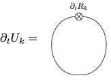
The flow of the effective potential is symbolized by

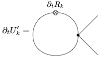
A \(\rho\)-derivative inserts external legs attached to a vertex,

and similarly,

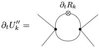
This is the perturbative Feynman diagram with the insertion of \(\partial_t R_k\). Renormalized vertices replace the bare vertices. The \(\partial_t R_k\) insertion removes divergencies from the momentum integral. The flow equation has the important property that only the couplings at a given scale \(k\) appear, not the bare couplings. The computation of a change of \(\Gamma_k[\Phi]\) only involves \(\Gamma_k[\Phi]\)!

Running coupling

The solution of the flow equation is easily found by integration. In a first step one writes \[\frac{d\lambda}{\lambda^2} = - d(1/\lambda) = \frac{N+8}{16\pi^2} d\ln(k),\] which integrates to \[\frac{1}{\lambda(k)}=\frac{1}{\lambda_\Lambda} + \frac{N+8}{16\pi^2}\ln(\Lambda/k).\] Finally the solution is \[\lambda(k) = \frac{\lambda_\Lambda}{1+\frac{(N+8)\lambda_\Lambda}{16\pi^2} \ln(\Lambda/k)}.\] As \(k\) decreases, \(\lambda(k)\) decreases.

Triviality

For any fixed \(\Lambda\) and \(\lambda_\Lambda>0\), one finds for \(k\to 0\) that \(\lambda(k\to 0)=0\).

The interaction vanishes in this limit and one ends up with a free theory. This is called “triviality”. One can use the flow equation in order to show triviality without the assumption of small \(\lambda\).

External momenta

Consider the momentum-dependent four-parent vertex \[\lambda_k(p_1,p_2,p_3,p_4) = \frac{\delta^4 \Gamma_k}{\delta \Phi(p_1)\delta \Phi(p_2) \delta \Phi^*(p_3)\delta \Phi^*(p_4)}\] (We omit the internal indices, e. g. \(N=1\).) In lowest order, the flow equation is given by a one-loop diagram.

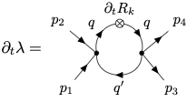
It involves the renormalized vertices \(\lambda_k(p_1,p_2,q,q')\) and \(\lambda_k(q,q',p_3,p_4)\). Momentum conservation at the vertices implies \[\begin{split} q-q' = p_1+p_2=p_3+p_4,\quad\quad\quad (q')^2 = (p_1+p_2-q)^2. \end{split}\] For \((p_1+p_2)^2=\mu^2\) and \(k^2 \ll \mu^2\), only momenta \(q^2<k^2\) or momenta \((q')^2\approx \mu^2\) contribute to the flow. This replaces in one of the propagators \(1/(k^2+m^2)\) by \(1/(\mu^2+m^2)\), leading to a suppression \(\propto k^2/\mu^2\). The flow effectively stops for \(k^2<\mu^2\). One can associate \[\lambda(\mu)\approx \lambda_{k^2= \mu^2}(0),\] where the left hand side represents the non-vanishing momenta at vanishing regulator scale \(k=0\), and the right hand side the vanishing momenta, at the regulator scale \(k^2=\mu^2\). Taking \(\lambda_R(\mu)=\lambda_{k=0}(\mu)\), one has \[\begin{split} \lambda_R(\mu) = \frac{\lambda_\Lambda}{1+\frac{(N+8)\lambda_\Lambda}{16\pi^2}\ln(\Lambda/\mu)}. \end{split}\] The flow equation describes now the dependence of the vertex on the scale of the external momenta. It is equivalent to the perturbative renormalization group.

Landau pole and “incomplete theories”

For the standard model, the Fermi scale \(\phi_0\) contributes an effective infrared cutoff. The renormalized coupling at \(k=\phi_0\) is measured by the observation of the mass of the Higgs boson \[m_H^2 = 2\lambda(\phi_0)\phi_0^2.\] We can use the flow equation in order to compute \(\lambda\) at shorter distance scales \(k>\phi_0\). We have \[\frac{1}{\lambda(k)}-\frac{1}{\lambda(\phi_0)} = -\frac{N+8}{16\pi^2}\ln(k/\phi_0),\] or \[\lambda(k)=\frac{\lambda(\phi_0)}{1-\frac{(N+8)\lambda(\phi_0)}{16\pi^2}\ln(k/\phi_0)}.\] We observe that \(\lambda(k)\) diverges at a Landau pole at a scale \(k_\text{Landau}\), i. e. \(\lambda(k)\to \infty\) for \(k\to k_\text{Landau}\).

One concludes that the \(\text{O}(N)\)-model with non-zero renormalized coupling \(\lambda_R(\mu)\) can not be continued to infinitely short scales. This is an “incomplete theory”. One finds similarly that the standard model is an incomplete theory. Some new physics is necessary at very short length scales in order to make the standard model a well-defined QFT. The Landau pole appears far beyond the Planck scale for gravity. The completion of the standard model could therefore be provided by quantum gravity, changing the flow of couplings for \(k>M_\text{Planck}\), where \(M_\text{Planck}\approx 10^{18}\) GeV.

Predictivity

Let us compute the flow equation for \(\nu=U^{\prime\prime\prime}(\rho_0)\). We neglect \(U^{(4)}(\rho)\) and higher \(\rho\)-derivatives. \[\begin{split} \partial_t U_k'''(\rho) &= -\frac{3}{16\pi^2k^2}\left[ \frac{(3U''+2\rho U''')^3}{(1+w_1)^4}+(N-1) \frac{(U'')^3}{(1+w_2)^4}\right]\\ & \quad- \frac{1}{16\pi^2}\left[\frac{5U'''(3U''+2\rho U'')}{(1+w_1)^3}+(N-1) \frac{U'''U''}{(1+w_2)^3} \right]. \end{split}\] With \(U''=\lambda, ~U'''\propto \lambda^3\), the leading term in an expansion in small \(\lambda\) is \[\begin{split} \partial_t\nu &= - \frac{3(N+26)\lambda^3}{16\pi^2k^2}. \end{split}\] For the dimensionless ratio \(\tilde \nu = \nu k^2\), one has \[\begin{split} \partial_t \tilde \nu = \beta_{\tilde\nu} = 2\tilde \nu- \frac{3(N+26)\lambda^3}{16\pi^2} . \end{split}\] The function \(\beta_{\tilde\nu}\) has a zero for \[\begin{split} \tilde \nu_* = \frac{3(N+26)\lambda^3}{32\pi^2k^2}. \end{split}\] Indicating the flow for decreasing \(k\) by arrows, one obtains the diagram

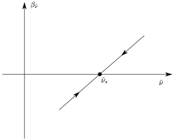
The solution of the flow equation attracts \(\tilde \nu\) to the partial-IR fixed point \(\tilde v_*\). For a given \(k\), this predicts \[\begin{split} \nu(k) &= \frac{3(N+26)\lambda(k)^3k^2}{32\pi^2}. \end{split}\] More precisely, one has \[\begin{split} \partial_t \left[ \frac{\tilde \nu}{\lambda^3} \right] &= 2 \left[ \frac{\tilde \nu}{\lambda^3} \right] - \frac{3(N+26)}{16\pi^2} - \frac{\tilde\nu}{\lambda^4}\partial_t\lambda \\ &= \left[2- \frac{N+8}{16\pi^2}\lambda\right]\frac{\tilde\nu}{\lambda^3}-\frac{3(N+26)}{16\pi^2}. \end{split}\] The effects of the running of \(\lambda\) can be neglected and one finds for the ratio \(z=\tilde\nu/\lambda^3\), \[\partial_t z = 2(z-z_*),\] with the fixed point value \(z_* = \tilde\nu_* / \lambda^3\). The solution is a power law behaviour \[z-z_* = c_0 \frac{k^2}{\Lambda^2}.\] This implies \[\tilde\nu-\tilde\nu_* = c_0 \lambda^3\frac{k^2}{\Lambda^2},\] or \[\nu = \frac{\tilde\nu_*}{k^2} + \frac{c_0\lambda^3}{\Lambda^2}.\] For \(k^2 \ll \Lambda^2\), the initial value (a bare coupling) \(\nu(\Lambda)\) that is specified by \(c_0\) plays no role. The flow “looses the memory about its microphysics”.

This happens to all couplings except for the two renormalizable couplings \(\lambda_R\) and \(\rho_{0,R}\). All other couplings can be produced, and can ultimately be expressed in terms of \(\lambda_R\) and \(\rho_{0,R}\)!