Quantum field theory 2, lecture 18

Functional renormalization

We have seen that loop integrals often contain ultraviolet divergencies if the UV cutoff is moved to infinity, or infrared divergencies if a particle mass scale is sent to zero. Quantities dominated by infrared fluctuations become predictable in terms of a few “renormalised couplings”. This idea is the central point why quantum field theory has predictive power. Rather than dealing with this idea in a technical fashion, we will develop the concepts that explain why “technical miracles” (as the cancellation of the divergencies) occur in perturbation theory. This is done by introducing functional renormalization as developed by Wilson, Wegner, Symanzik, Kadanoff and others.

The main idea is to relate the microphysical laws encoded by the classical action \(S[\phi]\) to the macrophysical laws that can be extracted from the quantum effective action \(\Gamma[\Phi]\). This is done in a continuous way by the effective average action \(\Gamma_k[\Phi]\), which intuitively describes the laws at a length scale \(1/k\). This effective average action interpolates smoothly between the classical action (at \(k=\Lambda\) or \(k\to\infty\)) and the quantum effective action (at \(k=0\)). In this way, the effect of fluctuations is included incrementally. The way in which \(\Gamma_k[\Phi]\) depends on \(k\) is described by a so-called “flow-equation” or “renormalization group equation”.

Intuitively, the effective average action includes the effects of all fluctuations with Ecuclidean momenta \(p\) larger than \(k\), \(p^2 > k^2\), but does not include those with smaller momenta, \(p^2<k^2\). The small momentum fluctuations are “cut off” by an infrared regulator function.

We discuss the principle ideas of functional renormalization using abstract index notation for bosonic theories. Extensions to theories with fermions, gauge fields and so on are also available.

Regulator

In order to implement these ideas, we add to the action a regulator piece \[\Delta S_k[\phi] = \frac{1}{2} R_{k\alpha\beta} \phi^\alpha \phi^\beta.\] Typically, the role of \(R_{k\alpha\beta}\) is to regularize fluctuations in the infrared, for example it can in the form of a mass term \[\Delta S_k[\phi] = \int_x \left\{ \frac{1}{2} k^2 \phi_n(x) \phi_n(x) \right\}.\] However, we keep the form of \(R_{k\alpha\beta}\) open for the moment. In most applications it vanishes in one limit, and becomes large in another.

Generating functionals in presence of regulator

We can now repeat all definitions for generating functionals in the presence of a regulator for \(k>0\). The Schwinger functional becomes \(k\)-dependent, \[\begin{split} e^{W_k[J]} = \int D\phi \, \exp\left(-S[\phi]-\Delta S_k[\phi]+ J_\alpha \phi^\alpha \right). \end{split}\] Only the action, not the construction, is modified. The same holds for the Legendre transform \[\tilde{\Gamma}_k [\Phi] = \sup_J \left( J_\alpha \Phi^\alpha - W_k[J] \right). %\label{eq:defGammaTilde}\] The relation between \(\Phi\) and \(J\) depends now on \(k\), \[\frac{\delta W_k[J]}{\delta J(x)} = \Phi(x),\quad\quad\quad \frac{\delta \tilde \Gamma_k[\Phi]}{\delta \Phi(x)} = J(x), %\label{eq:wGammafirstder}\] since \(W_k[J]\) and \(\tilde \Gamma_k[\Phi]\) depend on \(k\).

Flowing action

For the definition of the flowing action or effective average action \(\Gamma_k[\Phi]\), we subtract from \(\tilde \Gamma_k[\Phi]\) the regulator piece, now in terms of \(\Phi(x)\), \[\Gamma_k[\Phi] = \tilde \Gamma_k[\Phi] - \Delta S_k[\Phi] = \tilde \Gamma_k[\Phi] - \frac{1}{2} R_{k\alpha\beta} \Phi^\alpha \Phi^\beta.\] In this notation one can write \[\frac{\delta \Gamma_k[\Phi]}{\delta \Phi^\alpha} = J_\alpha- R_{k\alpha\beta} \Phi^\beta.\]

Background field identity

Inserting these definitions, one obtains \[\exp\left(-\Gamma_k[\Phi] \right) = \int D\phi'~\exp\left(-S[\Phi+\phi'] + \frac{\delta \Gamma_k[\Phi]}{\delta \Phi^\alpha} \phi^{\prime\alpha} - \frac{1}{2} R_{k\alpha\beta} \phi^{\prime\alpha} \phi^{\prime\beta} \right)\] Interestingly, the infrared regulator only acts on the fluctuations \(\phi^{\prime\alpha}=\phi^\alpha-\Phi^\alpha\).

Limit of large regulator scale

From the background field identity one can derive a few important results concerning limits of the effective average action. Consider first the limit of very large \(k\) and assume \[R_{k\alpha\beta} \to k^2 \delta_{\alpha\beta} \quad\quad\quad (k\to\infty).\] This is indeed the case for the constant or mass-type regulator \(k^2\). In this case the regulator part suppresses all fluctuations in the functional integral, and forms a representation of a functional Dirac delta, \[\delta[\phi] = \lim_{k\to\infty} \exp\left( -\frac{1}{2} R_{k\alpha\beta} \phi^{\alpha} \phi^{\beta} - c_k \right).\] The constant \(c_k\) is not important for most purposes. With the functional Dirac delta and the background field identity one obtains \[\lim_{k\to\infty} \Gamma_k[\Phi] + c_k = S[\Phi].\] For large regulator scale, the effective average action approaches the microscopic action!

If one wants to start at some large scale \(k=\Lambda\), one can often work with \(\Gamma_\Lambda[\Phi]\) being equal to \(S[\Phi]\) plus one-loop terms, where the latter are calculated in the presence of the regulator.

Limit or small regulator scale

The limit of small regulator scale is very easily taken, at least on the formal level. Here the regulator is supposed to vanish, \[R_{k\alpha\beta} \to 0 \quad\quad\quad (k\to 0).\] This ensures that the effective average action approaches the quantum effective action, \[\lim_{k\to 0}\Gamma_k[\Phi] = \Gamma[\Phi].\] In this lmimit, all fluctuations get included in the quantum effective action.

The flowing action \(\Gamma_k[\Phi]\) interpolates between the microscopic action \(S[\Phi]\) and the macroscopic quantum effective action \(\Gamma[\Phi]\).

Some remarks

1. In practice, there is often a finite microscopic (UV) scale \(\Lambda\). Instead of taking the limit \(k\to \infty\), one sets \(k\to \Lambda\). Thus, \(\Gamma_\Lambda[\Phi]\) can be associated with the microscopic action (though in principle, the first step is to compute \(\Gamma_\Lambda[\Phi]\) from \(S[\phi]\)).

2. Symmetries of \(\Gamma_k\)[]: All symmetries of \(S[\phi]+\Delta S_k[\phi]\) (in absence of anomalies) or of \(\Gamma_\Lambda[\phi]\) and \(\Delta S_k[\phi]\) are also symmetries of \(\Gamma_k[\Phi]\). Sometimes the infrared regulator can violate certain symmetries.

3. Effective laws: \(\Gamma_k[\Phi]\) encodes the effective laws at the momentum scale \(k\), i. e. at the length scale \(1/k\). Thus, the flow to lower \(k\) can intuitively be understood as “zooming out” with a microscope that enables to adjust to variable resolutions. When fluctuations \(p^2<k^2\) are not yet included, \(\Gamma_k[\Phi]\) describes a situation analogous to an experiment with a finite probe size \(1/k\). Therefore \(\Gamma_k[\Phi]\) is called the “flowing action”.

4. To take into account fluctuations only down to a certain momentum \(k\) can also be interpreted as averaging of fields, taking into account all interactions within a range \(1/k\). Therefore, one talks about the “effective average action”.

Exact flow equation

The flowing action obeys an exact flow equation (C. Wetterich 1993), \[\partial_k\Gamma_k[\Phi] = \frac{1}{2}\text{Tr} \left\{ (\Gamma^{(2)}[\Phi]+R_k)^{-1}\partial_k R_k \right\}.\] It is a functional differential equation and both \(\Gamma_k[\Phi]\) and \(\Gamma_k^{(2)}[\Phi]\) are functionals of the field expectation values \(\Phi^\alpha = \langle \phi^\alpha \rangle\).

Beyond purely bosonic theories, the trace is replaced by a supertrace operation which includes an additional sign for fermionic fields.

Derivation of the flow equation

In order to derive the exact flow equation we use several steps.

1. We first show that the definition of \(\tilde \Gamma_k[\Phi]\) as a Legendre transform of \(W_k[J]\), \[\tilde \Gamma_k[\Phi] = \sup_J \left( J_\alpha \Phi^\alpha - W_k[\Phi] \right)\] implies \[\partial_k \tilde \Gamma_k[\Phi] = -\partial_kW_k[J].\] This holds as one can see by carefully taking derivatives using the chain rule, \[\partial_k \tilde\Gamma_k[\Phi]{\big |}_\Phi = -\partial_k W_{k}[J]{\big |}_J - \frac{\delta W_k[J]}{\delta J_\alpha}\partial_k J_\alpha{\big |}_{\Phi} + \Phi^\alpha\partial_k J_\alpha {\big |}_{\Phi} = -\partial_k W_{k}[J]{\big |}_J.\]

2. Now we evaluate this further \[\begin{split} -\partial_k W_k[J] &= -\partial_k \ln \int D\phi~\exp\left(-S[\phi]-\Delta S_k[\phi] + J_\alpha \phi^\alpha \right)\\ &= \frac{1}{Z} \int D\phi~\exp\left(-S[\phi]-\Delta S_k[\phi] + J_\alpha \phi^\alpha \right)\partial_k\Delta S_k[\phi]\\ &= \partial_k\langle \Delta S_k[\phi]\rangle, \end{split}\] where we used that only \(\Delta S_k[\phi]\) depends on \(k\).

3. The formula for the propagator is derived as follows. We start from the definition \[G^{\alpha\beta} = \langle \phi^\alpha \phi^\beta\rangle - \langle \phi^\alpha \rangle\langle\phi^\beta\rangle,\] which can be rewritten to \[\langle \phi^\alpha \phi^\beta\rangle = G^{\alpha\beta}+\Phi^\alpha \Phi^\beta.\] Note that for bosonic fields \(G^{\alpha\beta} = G^{\beta\alpha}\). This results in \[\partial_k\tilde\Gamma_k[\Phi] = \frac{1}{2} (\partial_k R_{k\alpha\beta}) G^{\alpha\beta} + \frac{1}{2}(\partial_k R_{k\alpha\beta}) \Phi^\alpha \Phi^\beta.\] For \(\Gamma_k[\Phi] = \tilde\Gamma_k[\Phi]-\Delta S_k[\Phi]\) we find \[\begin{split} \partial_k \Gamma_k[\Phi] &= \frac{1}{2} (\partial_k R_{k\alpha\beta}) G^{\alpha\beta} = \frac{1}{2}\text{Tr}\{G \partial_k R_k \}. \end{split}\] Here, \[G^{\alpha\beta} = \frac{\delta^2 W_k[J]}{\delta J_\alpha\delta J_\beta},\] is the propagator matrix in the presence of the infrared regulator at scale \(k\). It depends on sources or fields.

4. Let us now rewrite the propagator part further. We employ the general matrix identity for Legendre transforms \[G^{\alpha\beta} (\tilde \Gamma_k^{(2)})_{\beta\gamma} = G^{\alpha\beta} (\Gamma_k^{(2)}+R_k)_{\beta\gamma} = \delta^\alpha_{~\gamma}.\] This is easily shown, \[\frac{\delta^2 }{\delta J_\alpha\delta J_\beta} W_k[J] \frac{\delta^2}{\delta \Phi^\beta\delta \Phi^\gamma} \tilde\Gamma_k[\Phi] = \frac{\delta \Phi^\beta}{\delta J_\alpha} \frac{\delta J_\gamma}{\delta \Phi^\beta} = \frac{\delta J_\gamma}{\delta J_\alpha} = \delta^\alpha_{~\gamma}.\] This yields the final form of the closed flow equation and concludes the proof.

Rewriting the flow equation

A dimensionless form of the flow equation is obtained by multiplying with \(k\) and by defining \(\partial_t= k\partial_k\), \[\partial_t\Gamma_k[\Phi] = \frac{1}{2}\text{Tr} \left\{ (\Gamma^{(2)}[\Phi]+R_k)^{-1}\partial_t R_k \right\}.\] Here \(t = \ln(k/\Lambda)\) is sometimes called RG time, but has nothing to do with physical time.

Another rewriting is sometimes useful, \[\partial_t \Gamma_k[\Phi] = \frac{1}{2}\text{Tr} \left\{ \tilde \partial_t \ln (\Gamma^{(2)}_k[\Phi]+R_k) \right\},\] with the formal scale derivative \(\tilde\partial_t\) which hits only the regulator term \(R_k\). Recalling the one-loop formula \[\Gamma_\text{1-loop}[\Phi] = \frac{1}{2}\text{Tr}\left\{ \ln S^{(2)}[\Phi] \right\},\] one sees the close correspondence to perturbation theory and Feynman graphs. A Feynman diagram for the flow equation can be given as

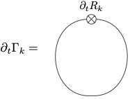
The line represents an exact and field-dependent propagator.