Quantum field theory 1, lecture 09

Perturbation theory

Let us now consider for simplicity the simple scalar theory (\(N=1\)) with an interaction term \(( \lambda / 4!) \phi^4\) and write the partition function formally in the form \[\begin{split} Z[J] = & \int D\phi \, \exp\left(-\frac{\lambda}{4!} \int_\mathbf{z} \phi(\mathbf{z}) \phi(\mathbf{z}) \phi(\mathbf{z}) \phi(\mathbf{z})\right) \exp\left(-S_2[\phi] + \int_\mathbf{x}J(\mathbf{x}) \phi(\mathbf{x}) \right) \\ = & \exp\left({-\frac{\lambda}{4!} \int_\mathbf{z} \frac{\delta}{\delta J(\mathbf{z})} \frac{\delta}{\delta J(\mathbf{z})} \frac{\delta}{\delta J(\mathbf{z})} \frac{\delta}{\delta J(\mathbf{z})}} \right) \int D\phi \exp\left({-S_2[\phi] + \int_\mathbf{x}J(\mathbf{x}) \phi(\mathbf{x})}\right) \\ = & \text{const} \times \exp\left({-\frac{\lambda}{4!} \int_\mathbf{z} \frac{\delta}{\delta J(\mathbf{z})} \frac{\delta}{\delta J(\mathbf{z})} \frac{\delta}{\delta J(\mathbf{z})} \frac{\delta}{\delta J(\mathbf{z})}} \right) \, \exp\left({ \frac{1}{2}\int_{\mathbf{x},\mathbf{y}} J(\mathbf{x}) G(\mathbf{x},\mathbf{y}) J(\mathbf{y})} \right). \end{split} \nonumber\] The two exponentials can be expanded into their Taylor series. Specifically the expansion of the first exponential leads to a perturbative series in the coupling constant \(\lambda\). The constant term in the last line contains is independent of the source \(J\) but depends on temperature \(T\) so that we will have to partly take it into account for discussing thermodynamics.

Feynman diagrams for the partition function

Terms in the perturbative series for the partition function \(Z[J]\) and for correlation functions that are obtained as functional derivatives of \(Z[J]\) have a nice graphical representation in terms of Feynman diagrams. This arises here in a purely classical statistical setup, but works very similar for quantum fields as we will see later on.

Expanding the two exponential functions in the partition function, one finds \[\label{eq:PartitionFunctionPerturbationTheory} Z[J] = \text{const} \times \sum_{V=0}^\infty \frac{1}{V!} \left( -\frac{\lambda}{4!} \int_\mathbf{z} \frac{\delta^4}{\delta J(\mathbf{z})^4} \right)^V \sum_{P=0}^\infty \frac{1}{P!} \left( \frac{1}{2}\int_{\mathbf{x},\mathbf{y}} J(\mathbf{x}) \, G(\mathbf{x}, \mathbf{y}) \, J(\mathbf{y}) \right)^P \; ,\] where the index \(V\) can be understood as couting the number of four-vertices and \(P\) as counting the number of propagator lines. Once the functional derivatives associated with every vertex have been done, we have \(2P-4V\) powers of the source \(J(\mathbf{x})\) left. When we later want to calculate correlation functions by taking functional derivatives of the partition functions, the functional derivatives act on these source terms.

Graphical representation

It is convenient to introduce a graphical representation for objects that appear in a systematic manner in the terms of the perturbative series \(\eqref{eq:PartitionFunctionPerturbationTheory}\). The three building blocks are composed of the propagator \(G(\mathbf{x}, \mathbf{y})\), the sources \(J(\mathbf{x})\) and the four-vertex associated to the coupling constant \(\lambda\). We introduce a graphical representation where propagators correspond to lines, sources to endpoints, and interaction terms to vertices where four lines meet,

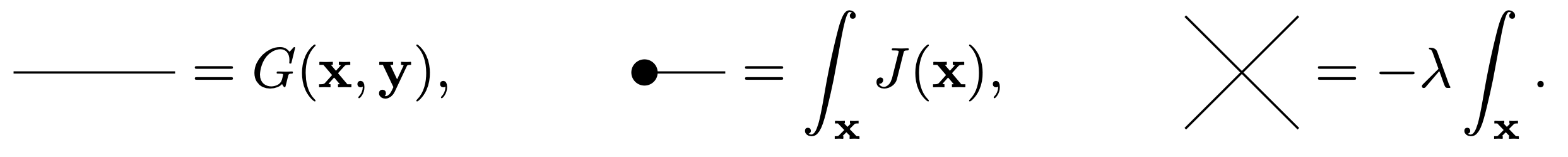
The corresponding Feynman rules are rather simple for this model: each propagator gets attached with its two ends to a source or a vertex.

Terms without vertices

As an exercise let us consider a few diagrams out of the infinite series generated by the expansion \(\eqref{eq:PartitionFunctionPerturbationTheory}\). Consider e.g. the term corresponding to \(V=0\) and \(P=1\),

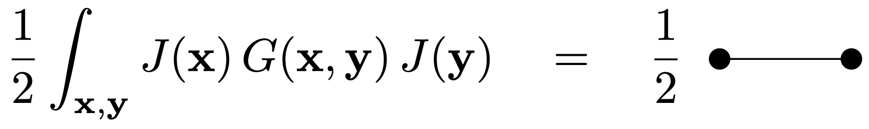
This has no vertices can can be seen as a contribution at lowest order \(\lambda^0\) in the perturbative expansion. For \(V=0\) and larger values of \(P\), we get products of these terms which give a factorized form of the partition function. For example, for \(V=0\) and \(P=3\) we get

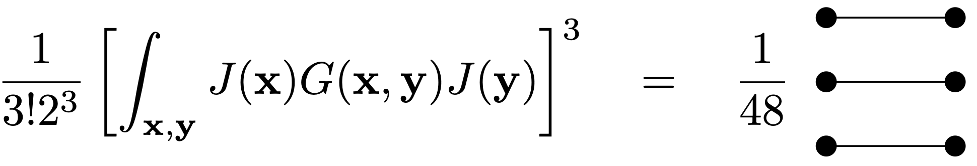
Like this on can go on and finds \(2P\) sources in each term. The correlation functions following from these terms by taking functional derivatives with respect to the sources \(J\) are obeying Wicks theorem. This means that two

Diagram with one vertex but no sources left

For positives values of \(V\) one obtains from the expansion of the first exponential in eq. \(\eqref{eq:PartitionFunctionPerturbationTheory}\) for each power of \(\lambda\) four functional derivatives with respect to the sources \(J(\mathbf{z})\). This reduces the number of sources to \(2P-4V\).

For example, for \(V=1\) and \(P=2\) one obtains the expression

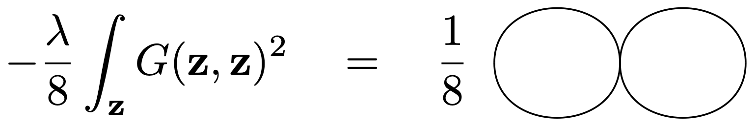
This is a diagram with two loops, but no source terms left, so it will not contribute to any correlation function. This is called a vacuum diagram.

Diagrams contributing to two-point function

For \(V=1\) and \(P=3\) there are two type of diagrams appearing,

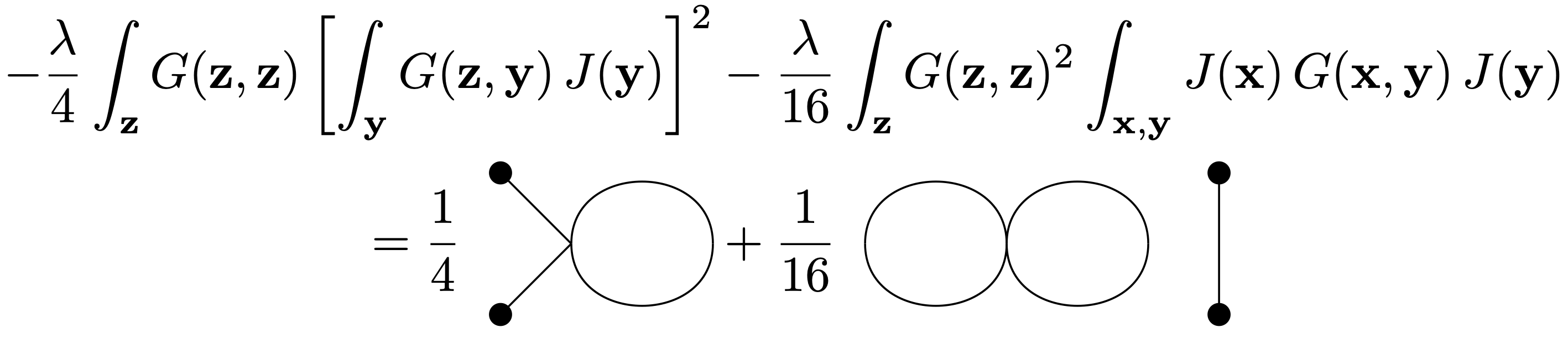
Here the first diagram gives a non-trivial and connected contribution to the two-point correlation function with one loop. In contrast, the second diagram falls into a product of two disconnected pieces with the first being a vacuum diagram and the second a contribution to the two-point function.

Tree diagram with one vertex

For \(V=1\) and \(P=4\) there are a couple of diagrams, but one of them has the form

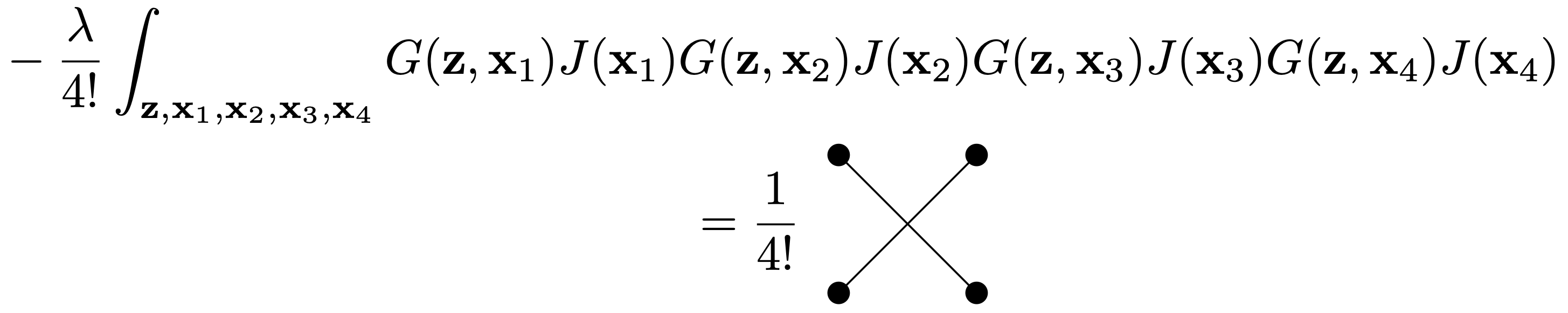
Taking here four functional derivatives with respect to the sources leads to a contribution to the four-point correlation function that does not factorize into two-point functions. It describes a proper correlation between all four points.

Different kinds of diagrams

In these three examples we already encountered two important classes of diagrams. There exist diagrams which do not include closed cycles or loops and are usually called tree diagrams whereas diagrams including closed cycles are call loop diagrams. Furthermore, there are diagrams as in \(\eqref{eq:PartitionFunctionV0P1}\), \(\eqref{eq:PartitionFunctionV1P2}\) and the first diagram in \(\eqref{eq:PartitionFunctionV1P3}\) which are connected whereas the second diagram in \(\eqref{eq:PartitionFunctionV1P3}\) is disconnected. A further distinction arises between vacuum diagrams and diagrams that actually contribute to correlation functions.

Divergences

At first sight, it might seem diagrams such as \(\eqref{eq:PartitionFunctionV1P2}\) contain divergencies associated to the coincidence limit of the propagator as well as an integral over the whole space. As we will realise later, these kind of diagrams (in QFT called ‘vacuum bubbles’) do not contribute to correlation functions. In contrast, loop diagrams such as the first diagram in \(\eqref{eq:PartitionFunctionV1P3}\) do contribute to correlation functions and the associated ultraviolet divergence from \(G(\mathbf{z}, \mathbf{z})=\infty\) is handled later on by renormalisation.

Generating functionals

Schwinger functional and connected diagrams

It is often useful to consider instead of the partition function \(Z[J]\) the Schwinger functional \(W[J]\) defined through \[Z[J] = e^{W[J]}.\] The expectation value is simply obtained through \[\langle \phi(\mathbf{x}) \rangle = \frac{\delta}{\delta J(\mathbf{x})} W[J] = \frac{1}{Z[J]} \frac{\delta}{\delta J(\mathbf{x})} Z[J].\] The second functional derivative yields the connected two-point correlation function \[\begin{split} \mathcal{G}(\mathbf{x}, \mathbf{y}) =\frac{\delta^2}{\delta J(\mathbf{x})\delta J(\mathbf{y})} W[J] & = \frac{1}{Z[J]}\frac{\delta^2}{\delta J(\mathbf{x})\delta J(\mathbf{y})} Z[J] - \frac{1}{Z[J]^2}\frac{\delta}{\delta J(\mathbf{x})} Z[J] \frac{\delta}{\delta J(\mathbf{y})} Z[J] \\ & = \langle \phi(\mathbf{x}) \phi(\mathbf{y}) \rangle - \langle \phi(\mathbf{x}) \rangle \langle \phi(\mathbf{y}) \rangle . \end{split}\nonumber\] This connected correlation function the usually vanishes at large separation. Note that the full correlation function \(\mathcal{G}\) and its counterpart \(G\) for the free theory agree at the leading order \(\lambda^0\) in a perturbative expansion but differ beyond that.

Connected three-point correlation function

In a similar way one can now determine third functional derivatives, \[\begin{split} & \langle \phi(\mathbf{x}) \phi(\mathbf{y}) \phi(\mathbf{z}) \rangle_c = \frac{\delta^3}{\delta J(\mathbf{x})\delta J(\mathbf{y}) \delta J(\mathbf{z})} W[J] = \langle \phi(\mathbf{x}) \phi(\mathbf{y}) \phi(\mathbf{z}) \rangle \\ & - \langle \phi(\mathbf{x}) \phi(\mathbf{y}) \rangle \langle \phi(\mathbf{z}) \rangle - \langle \phi(\mathbf{y}) \phi(\mathbf{z}) \rangle \langle \phi(\mathbf{x}) \rangle - \langle \phi(\mathbf{z}) \phi(\mathbf{x}) \rangle \langle \phi(\mathbf{y}) \rangle + 2 \langle \phi(\mathbf{x}) \rangle \langle \phi(\mathbf{y}) \rangle \langle \phi(\mathbf{z}) \rangle, \end{split}\nonumber\] which is known as the connected three-point correlation function. Note that for vanishing expectation value, the connecetd three-point correlation function equals the full three-point correlation function.

Connected four-point correlation function

The four point function can be worked out in a similar way. One finds \[\begin{split} \langle\phi(\mathbf{x})\phi(\mathbf{y})\phi(\mathbf{z})\phi(\mathbf{w}) \rangle_c = \frac{\delta^4 W}{\delta J(\mathbf{x}) \delta J(\mathbf{y}) \delta J(\mathbf{z}) \delta J(\mathbf{w})} &= \langle \phi(\mathbf{x}) \phi(\mathbf{y}) \phi(\mathbf{z}) \phi(\mathbf{w}) \rangle\\ & - \langle\phi(\mathbf{x})\phi(\mathbf{y}) \rangle\langle \phi(\mathbf{z})\phi(\mathbf{w}) \rangle-\langle\phi(\mathbf{x})\phi(\mathbf{z}) \rangle\langle\phi(\mathbf{y})\phi(\mathbf{w}) \rangle\\ &-\langle\phi(\mathbf{x})\phi(\mathbf{w}) \rangle\langle\phi(\mathbf{y})\phi(\mathbf{z}) \rangle+\text{terms involving }\langle\phi \rangle . \end{split}\] For vanishing expectation value, the connected four-point function subtracts from the four point function the “unconnected parts". In this way one can go on and decompose all correlation functions in connected and disconnected parts. It turns out that in many physics applications one actually is interested in connected terms only.

In the context of finite dimensional random variables, correlation functions are known as moments and connected correlation functions are known as cumulants.

Thermodynamic significance

Recall that in our present context the partition function is for \(J=0\) and with \(\beta=1/T\) \[Z[0] = e^{W[0]} = e^{-\beta F(T)} = \text{Tr} \left\{ e^{-\beta H} \right\}.\] Up to an additive constant the Schwinger functional at vanishing source is the free energy devided by the temperature, \[W[0] = - F(T) / T = - (E - T S)/T.\] From the free energy one can obtain for example the entropy according to \(S=-\partial F / \partial T\) or the expectation value of energy as \(E=F+TS\). Of course, to calculate this we need to follow carefully the dependence on temperature \(T\). This can be generalized to situations with more conserved quantum numbers, such as some particle number \(N\) coupled to a chemical potential \(\mu\). We will later also study the generalization to quantum statistics.

Partition function and Schwinger functional at vanishing source

We concentrate now first on the leading contribution at order \(\lambda^0\) to the partition function and Schwinger functional at vanishing source. From the evaluation of the Gaussian integral we find (still neglecting the contribution of conjugate momenta here) \[Z[0] = e^{W[0]} = \lim_{N\to \infty} (2\pi)^{N/2} \text{det}(D)^{-1/2},\] where \(D\) is the matrix inverse to the propagator function \(G(\mathbf{x}, \mathbf{y})\). The factors of \(2\pi\) can be dropped, they only lead to a numerical offset in \(W[0]\) that is independent of temperature. To evaluate the determinant we use the identity \[\ln( \det(D)) = \text{tr}\{ \ln(D) \}.\] The latter can be easily proven in case that \(D\) is diagonal and extended beyond that by the definition of the logarithm.

Loop expansion for Schwinger functional

This leads to \[W[0] = \text{const} - \frac{1}{2} \text{tr} \ln(D) .\] The second term can be graphically represented by a single closed loop. In a perturbative expansion we find that this gets supplemented by a two-loop term at order \(\lambda^1\), two possible tree-loop terms at order \(\lambda^2\) and so on, \[W[0] = \text{const} - \frac{1}{2} \text{tr}\left\{ \ln(D) \right\} + \mathcal{O}(\lambda) + \mathcal{O}(\lambda^2) + \ldots.\] While it is straight forward to write down the connected vacuum diagrams and also to write down corresponding integral expressions, it will be more work to properly evaluate them.

In the partition function \(Z[0] = \exp(W[0])\) we also get products of the connected diagrams through the expansion of the exponential and it is therefore given by a sum of all possible vacuum diagrams.

Perturbative expansion for two- and four-point functions

We can now go ahead and consider terms in the Schwinger functional \(W[J]\) that depend on the source. Because our theory is invariant under the \(Z_2\) symmetry \(\phi\to - \phi\), \(J\to - J\), there are only even orders in \(J\). We can write \[W[J] = W[0] + \frac{1}{2} \int_{\mathbf{x}, \mathbf{y}} J(\mathbf{x}) \mathscr{G}(\mathbf{x}, \mathbf{y}) J(\mathbf{y}) + \frac{1}{4!} \int_{\mathbf{x}_1, \mathbf{x}_2, \mathbf{x}_3, \mathbf{x}_4} J(\mathbf{x}_1) J(\mathbf{x}_2) J(\mathbf{x}_3) J(\mathbf{x}_4) \mathscr{V}(\mathbf{x}_1, \mathbf{x}_2, \mathbf{x}_3, \mathbf{x}_4) + \ldots,\] where \(\mathscr{G}(\mathbf{x}, \mathbf{y})\) is a connected two-point correlation function including perturbative corrections, \(\mathscr{V}(\mathbf{x}_1, \mathbf{x}_2, \mathbf{x}_3, \mathbf{x}_4)\) is a connected four-point correlation function including perturbative corrections and so on.

For the two-point function we find at order \(\lambda^0\) \[\mathscr{G}(\mathbf{x}, \mathbf{y}) = G(\mathbf{x} - \mathbf{y}),\] and this gets corrected by a one-loop term at order \(\lambda^1\), three different two-loop terms at order \(\lambda^2\) and so on.

Similarly, the four-point function has the leading contribution (a tree diagram) \[\mathscr{V}(\mathbf{x}_1, \mathbf{x}_2, \mathbf{x}_3, \mathbf{x}_4) = -\lambda \int d^d x \, G(\mathbf{x}_1-\mathbf{x}) G(\mathbf{x}_2-\mathbf{x}) G(\mathbf{x}_3-\mathbf{x}) G(\mathbf{x}_4-\mathbf{x}),\] and this gets supplemented by different one-loop terms at order \(\lambda\), two-loop terms at order \(\lambda^2\) and so on.